Dynamic programming algorithms#
This chapter introduces the notion of dynamic programming algorithms with the implementation of one algorithm of this kind, which calculates Fibonacci numbers. The historic hero introduced in these notes is Leonardo of Pisa, a.k.a. Fibonacci, who was one of the most prominent mathematicians of the Middle Ages.
Note
The slides for this chapter are available within the book content.
Historic hero: Fibonacci#
Leonardo of Pisa, a.k.a. Fibonacci (depicted in Fig. 39, was a mathematician. He first introduced in Europe the Hindu-Arabic number system, which is the numeral system that is commonly used worldwide even today. This introduction was possible thanks to the publication of his book in 1202, Liber Abaci (Book of Calculation in English) [Fib02]. The book describes how to use such a numeral system to address commerce situations and solve generic mathematical problems.
One of the main contributions of Fibonacci in his book was a small note about a particular infinite sequence of numbers named after him. The sequence described the number of male-female pairs of rabbits at a given month. The Fibonacci sequence and the numbers it contains (i.e. 1 1 2 3 5 8 13 21 34 55 …) have very peculiar properties studied in the past by mathematicians and historians of science. It is calculated with a straightforward (and recursive!) approach. The Fibonacci number at a particular month n is equal to the sum between the Fibonacci number at month n-1 and that at month n-2, as shown in Equation (1). As a side note, fib(0) and fib(1) are equal to 0 and 1, respectively.

Fig. 39 A portrait of Leonardo Pisano, also known as Fibonacci. Source: Wikimedia Commons.#
One of the most popular properties that Fibonacci did not mention in his book is the relation between the Fibonacci sequence and the golden ratio. Mathematically speaking, two quantities are in the golden ratio when their ratio is the same as the ratio of their sum to the larger quantity. Equation (2) defines this value, where quantity a is greater than quantity b.
While, at first sight, this seems quite a simple ratio, it is defined by an irrational number. Thus, in principle, this number sounds to be quite abstract and a purely mathematical notion. However, it is used and observed in several different domains, such as architecture (e.g. the Pantheon in Athens), arts (e.g. Leonardo’s drawings in De divina proportione), and nature (e.g. the arrangement of leaves in plants).
The Fibonacci sequence is somehow closely related to the golden ratio. Taking a number in the sequence and dividing it by the previous one in the same sequence will return an approximation of the golden ratio Φ, and the higher the numbers, the more precise is the value:
5 / 3 = 1.66666…
8 / 5 = 1.6
13 / 8 = 1.625
21 / 13 = 1.61538…
34 / 21 = 1.61904…
55 / 34 = 1.61764…
…
Remembering solutions to sub-problems#
In the previous chapter, we have introduced how the divide and conquer algorithms generally work. Four steps characterise them: the handling of one or more base cases, the divide phase, the conquer step (i.e. the recursive action) and combine operation. Furthermore, we have explicitly said that such an approach is, in most cases, more efficient than the more straightforward brute force approach, at least for solving computational problems that can be split into two or more smaller problems of the same type.
However, some computational problems present even additional characteristics. Sometimes, they can be split into sub-problems, but some of these sub-problems recur during the execution. This situation can even happen when we have to sort books. For instance, suppose we have the following list of books with six items to sort: list(["Coraline", "American Gods", "Neverwhere", "Neverwhere", "American Gods", "Coraline"]). The list contains two copies of the same book. In this case, the application of the divide step of the merge sort returns two sublists. Such lists contain, basically, different copies of the same books in a different order. The left list will be list(["Coraline", "American Gods", "Neverwhere"]), while the right list will be list(["Neverwhere", "American Gods", "Coraline"]). However, even if the order between the books in the two sublists is different, the final result will be the same, i.e. the two lists ordered.
In the merge sort, we call the algorithm recursively twice (in the conquer step), even if we could, in principle, run it just once, i.e. on the left list and then to reuse the positions obtained for the books in such list for positioning the books in the right list. This approach could avoid spending additional time ordering something that we have already learned how to order. To implement this approach, we need to use some mechanism to keep track of the operation we have already done. In this way, it would be possible to reuse a result of a previous problem again and directly, without any further calculation.
This kind of approach is known as dynamic programming. Dynamic programming works like the divide and conquer approach. It is an algorithmic technique that splits the original computational problem to solve in two or more smaller problems of the same type. However, differently from the divide and conquer, it stores the solutions to these subproblems for reusing them if they recur. Thus, when a problem recurs, one can look at the previously-computed solution and reuse it directly, usually saving a considerable amount of computation time.
The following (informal) steps can define the dynamic programming approach:
[base case: solution exists] return the solution calculated previously to the problem if this is the case; otherwise
[base case: address directly] address the problem directly on the input material if it is depicting an easy-to-solve problem; otherwise
[divide] split the input material into two or more balanced parts, each representing a sub-problem of the original one;
[conquer] run the same algorithm recursively for every balanced part obtained in the previous step;
[combine] reconstruct the final solution of the problem using the partial solutions obtained from running the algorithms on the smaller parts of the input material;
[memorise] store the solution to the problem to reuse if needed by other recursive calls.
In the next section, we show a divide and conquer implementation of a computational problem. Then, we show how a dynamic programming approach decreases the number of operations to execute to achieve the same outcome.
Fibonacci sequence#
In Section Historic hero: Fibonacci, we have introduced a particular sequence of integer numbers, i.e. the Fibonacci sequence, that has been used by Fibonacci himself for providing a theoretical and approximated way for describing the evolution of a population of rabbits during months. The sequence, of course, is composed of specific numbers, and the calculation of these numbers is the particular problem we want to solve in this section:
Computational problem
Calculate the Fibonacci number at one specific month.
As shown in Section Historic hero: Fibonacci, each number in the Fibonacci sequence is defined recursively as the sum of the previous two numbers in the same sequence. Thus, this definition seems to suggest that it would be possible to write a divide and conquer algorithm to address this problem effectively. In this case, we use, as base cases, the Fibonacci number calculated for the months 0 and 1 that returns 0 and 1, respectively. Fig. 40 shows the execution of an algorithm for calculating the Fibonacci number. In particular, it takes month 4 as input. Then, it executes recursively the same algorithm on smaller input data as defined by the definition of Fibonacci numbers until it reaches the base case.
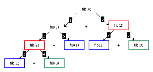
Fig. 40 The application of a divide and conquer approach for obtaining the 4th number in the Fibonacci sequence. We use coloured rectangles for showing identical calls to the Fibonacci algorithm with the same input. The numbers in the labels in the arrows indicate the sequence of execution of the various calls.#
As shown in Fig. 40, however, a lot of calculations are repeated multiple times. For instance, we run twice the executions of fib(2) and fib(0), while we execute three times fib(1). The implementation of this algorithm in Python, shown in Listing 48, is described by the following steps:
[base case] if the input number for which to find the Fibonacci number is 0 or 1, then return such input number; otherwise
[divide] obtain the two input numbers according to the Fibonacci definition;
[conquer] run the same algorithm recursively for each of the numbers obtained in the previous step;
[combine] sum the results of the partial solutions obtained by running the two executions of the algorithm recursively.
One can avoid repeating previously-computed solutions by adopting a dynamic programming approach. Part of the body of such an algorithm is very similar to the divide and conquer one mentioned above. The real difference is in two additional steps. In the first step, we check for the existence of a previously-calculated solution to the problem. The last step stores a new solution in memory for reusing it. Fig. 41 describes the algorithm’s execution to find the Fibonacci number at month 4 by reusing solutions stored in previous calls.
as part of the material of the course.# 1# Test case for the function
2def test_fib_dc(n, expected):
3 result = fib_dc(n)
4 if expected == result:
5 return True
6 else:
7 return False
8
9# Code of the function
10def fib_dc(n):
11 if n <= 0: # base case 1
12 return 0
13 elif n == 1: # base case 2
14 return 1
15 else: # recursive step
16 return fib_dc(n-1) + fib_dc(n-2)
17
18# Tests
19print(test_fib_dc(0, 0))
20print(test_fib_dc(1, 1))
21print(test_fib_dc(2, 1))
22print(test_fib_dc(7, 13))
There are several possible ways to store a solution to a problem. In this work, we suggest using a dictionary, specifying the key as the input number (i.e. the month) used to calculate the Fibonacci number and the value resulting from such a calculation. However, to implement the algorithm, we need to introduce some additional operations for managing dictionaries appropriately.
First of all, we need to check if such a dictionary includes already a particular key. We can use get method of dictionaries, i.e. <dictionary>.get(<key>), introduced in a previous chapter. This method will return a value if the dictionary contains the key; otherwise, it will return None. If needed, there is another way for checking the inclusion of a key in a dictionary, which is more efficient and even more natural to write and remember. We can use the comparison operations in and not in that we already introduced with strings. In particular, <key> in <dictionary> and <key> not in <dictionary> check if the specified key is or is not included in the dictionary, respectively.
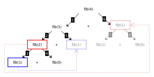
Fig. 41 The application of a dynamic programming approach for obtaining the 4th number in the Fibonacci sequence. We use coloured rectangles for showing identical calls to the Fibonacci algorithm with the same input. However, in this case, the result related to the transparent rectangles is obtained from previous computations of the same call (linked via the transparent dashed arrows). As a consequence of this reuse, we will not execute steps 7 and 8.#
In addition, we need to create this dictionary somehow when executing the algorithm so that the subsequent execution provided in the recursive step can be reused. Thus, generally speaking, the algorithm itself should:
initialises an empty dictionary as the very first step;
reusing such a dictionary when needed in any recursive application of the algorithm itself.
The function that implements the algorithm should be able to take the dictionary containing the solutions as input. In the first execution of the function, such a dictionary should be empty.
Now we have all the ingredients for creating the dynamic programming algorithm for calculating the Fibonacci number. Listing 49 introduces the related Python code, which implements the following steps:
[base case: solution exists] return the solution to the input number if available due to previous executions; otherwise
[base case: address directly] if the input number for which to find the Fibonacci number is 0 or 1, then return such input number; otherwise
[divide] obtain the two input numbers according to the Fibonacci definition;
[conquer] run the same algorithm recursively for each of the numbers obtained in the previous step;
[combine] sum the results of the partial solutions obtained by running the two executions of the algorithm recursively;
[memorize] store the sum into a dictionary using the original input number as the key.
as part of the material of the course.# 1# Test case for the function
2def test_fib_dp(n, d, expected):
3 result = fib_dp(n, d)
4 if expected == result:
5 return True
6 else:
7 return False
8
9# Code of the function
10def fib_dp(n, d):
11 # Checking if a solution exists
12 if n not in d:
13 if n <= 0: # base case 1
14 d[n] = 0
15 elif n == 1: # base case 2
16 d[n] = 1
17 else: # recursive step
18 # the dictionary will be passed as input of the recursive
19 # calls of the function
20 d[n] = fib_dp(n-1, d) + fib_dp(n-2, d)
21
22 return d.get(n)
23
24# Tests
25print(test_fib_dp(0, dict(), 0))
26print(test_fib_dp(1, dict(), 1))
27print(test_fib_dp(2, dict(), 1))
28print(test_fib_dp(7, dict(), 13))
Thus, if we have to run the algorithm for calculating the Fibonacci number at the 4th month, we just execute fib_dp(4, dict()), specifying an empty dictionary.
References#
Leonardo Fibonacci. Liber Abaci. Self-published, 1202. URL: https://bibdig.museogalileo.it/tecanew/opera?bid=1072400&seq=1.