Backtracking algorithms#
This chapter introduces an algorithmic technique used in constrained computational problems. Typical problems of this kind are those related to the resolution of abstract strategy board games, such as the peg solitaire. The historic hero introduced in these notes is AlphaGo, an artificial intelligence developed by Google DeepMind to play Go.
Note
The slides for this chapter are available within the book content.
Historic hero: AlphaGo#
AlphaGo (shown in Fig. 47) is an artificial intelligence developed by Google DeepMind for playing a particular board game, i.e. Go. As introduced in one of the first chapters, Go is an ancient abstract strategy board game. Due to its ample solution space, it is mainly known for being very complex to play by a computer.

Scientists developed several artificial intelligence applications to play Go automatically in the past. However, all of them showed their limits when tested with human expert players. Before 2016, no Go software was able to beat a human master. The approach adopted by those systems, even if sophisticated, was not enough for emulating the skills of expert human players.
In 2015, a particular department within Google declared to have developed the best artificial intelligence for playing Go and suggested testing it in an international match against one of the greatest Go players in Europe, Fan Hui. At the time of the game, Fan Hui was a professional two dan player (out of 9 dan). The match was in five sessions, and a player had to win at least three sessions out of five for winning the game. AlphaGo beat Fan Hui 5-0 and has become the first artificial intelligence to beat a professional human player. The outcomes of the match were announced in January 2016 simultaneously with the publication of the Nature article explaining the algorithm [SHM+16].
In March 2016, AlphaGo was engaged against Lee Sedol, a professional nine dan South Korean Go player, one of the best players in the world. All five sessions of the match were broadcast live in streaming video to allow people to follow the various games. AlphaGo beat Lee Sedol 4-1. Finally, in May 2017, AlphaGo was involved in a match in three sessions against the top-ranked player, the Chinese Ke Jie. Even this time, AlphaGo beat Ke Jie 3-0. After that, Google DeepMind decided to retire AlphaGo definitely from the scenes due to this match.
Several professional players have stated that AlphaGo seemed to use quite new moves if compared with the other professional players. As a consequence of its results and in several secondary games, Alpha Go gained recognition as a professional nine dan player by the Chinese Weiqi Association.
A final article about the latest evolution of the system, AlphaGo Zero, was published in Nature on the 18th of October 2017 [SSS+17]. In this article, the authors introduce the best version of AlphaGo that they have developed. The Alpha Go creators trained this new version without using any match between human champions archived in the past, as they did for training AlphaGo. In particular, they trained it against itself, and it reached a superhuman performance after only 40 days of self-training. As a result, the new AlphaGo Zero beat AlphaGo 100-0.
Tree of choices#
Usually, all the algorithms for finding a solution to abstract strategy board games use a tree, where each node represents a possible move on the board. Thus, the idea is that one comes to a particular node after executing a precise sequence of moves. Then, one can have an additional set of possible valid moves from that node to approach the solution. But, of course, to choose a particular move, one should also check if executing that move could bring a solution to our problem or it lands at a dead-end. In this latter case, one could reconsider some previous choices and, eventually, change strategy looking for some other, more promising, moves to follow.
Technically speaking, this approach is called backtracking in the Computational Thinking domain. In practice, backtracking algorithms try to solve a particular computational problem by identifying possible candidate solutions incrementally. Moreover, it abandons partial candidates once it is clear that they will not be able to solve the problem. The usual steps of a backtracking algorithm can be defined as follows, and consider a particular node of the tree of choices as input:
[leaf-win] if the current node is a leaf, and it represents a solution to the problem, then return the sequence of all the moves that have generated the successful situation; otherwise,
[leaf-lose] if the current node is a leaf, but it is not a solution to the problem, then return no solution to the parent node; otherwise,
[recursive-step] apply the whole approach recursively for each child of the current node until one of these recursive executions returns a solution. If none of them provides a solution, return no solution to the parent node of the current one.
In the next section, we illustrate the application of this technique for solving a particular board game: peg solitaire.
Peg solitaire#
Peg solitaire is a board game for one person only, which involves the movement of some pegs on board containing holes. Usually, in the starting situation, the board contains pegs everywhere except for the central position, which is empty. While there are different standard shapes for the board of the game, as illustrated in Fig. 48 – the classic board is the English one (the number 4 in Fig. 48).
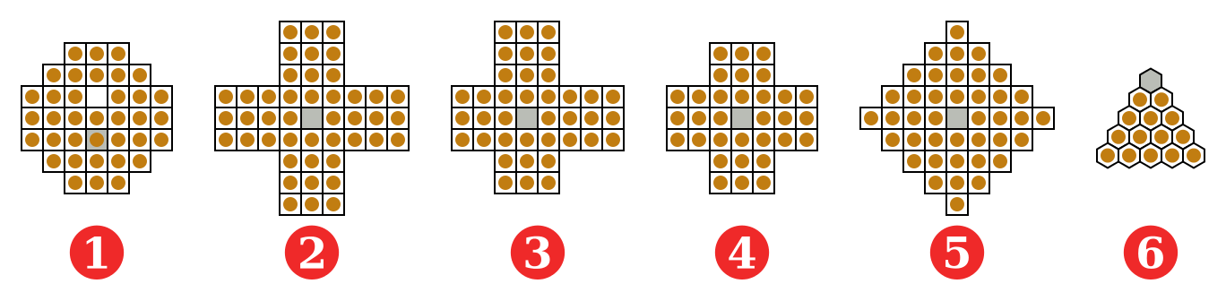
Fig. 48 Possible standard shapes for the board of the peg solitaire – the number 4 is the English one. Figure by Julio Reis, source: Wikimedia Commons.#
The game’s goal is to come to the opposite of the starting situation: the whole board must be full of holes except the central position, which must contain a peg. It is possible to repeatedly apply the same rule to reach this goal: to move a peg orthogonally over an adjacent peg into a hole and remove the jumped peg from the board. Fig. 49 illustrates an example of valid moves.

Fig. 49 An example of two consecutive and valid moves on an English board. Source: University of Waterloo.#
The computational problem we want to address in this chapter can be defined as follows:
Computational problem
Find a sequence of moves to solve the peg solitaire.
A reasonable approach for finding a solution to this computational problem is based entirely on backtracking. In particular, we should develop it according to the following steps:
[leaf-win] if the last move has brought to a situation where there is only one peg, and it is in the central position, then a solution has been found, and the sequence of moves executed for coming to this solution is returned; otherwise,
[leaf-lose] if the last move has brought to a situation where there are no possible moves, then recreate the previous status of the board as if we did not execute the previous move, and return no solutions; otherwise,
[recursive-step] apply the algorithm recursively for each possible valid move executable according to the board’s current status until one of these recursive executions of the algorithm returns a solution. If none of them provides a solution, recreate the previous status of the board as if we did not execute the last move and return no solutions.
The idea is to start with the initial configuration of the board as the root of a tree of moves. Then, we consider all the possible configurations reachable from such a root after a valid move, and so on. This process, in practice, would allow us to describe all the possible scenarios with quite a big tree. However, it is worth mentioning that visiting all the possible configurations is unnecessary. Instead, the algorithm can terminate with success once it reaches a final winning configuration, as summarised in Fig. 50.
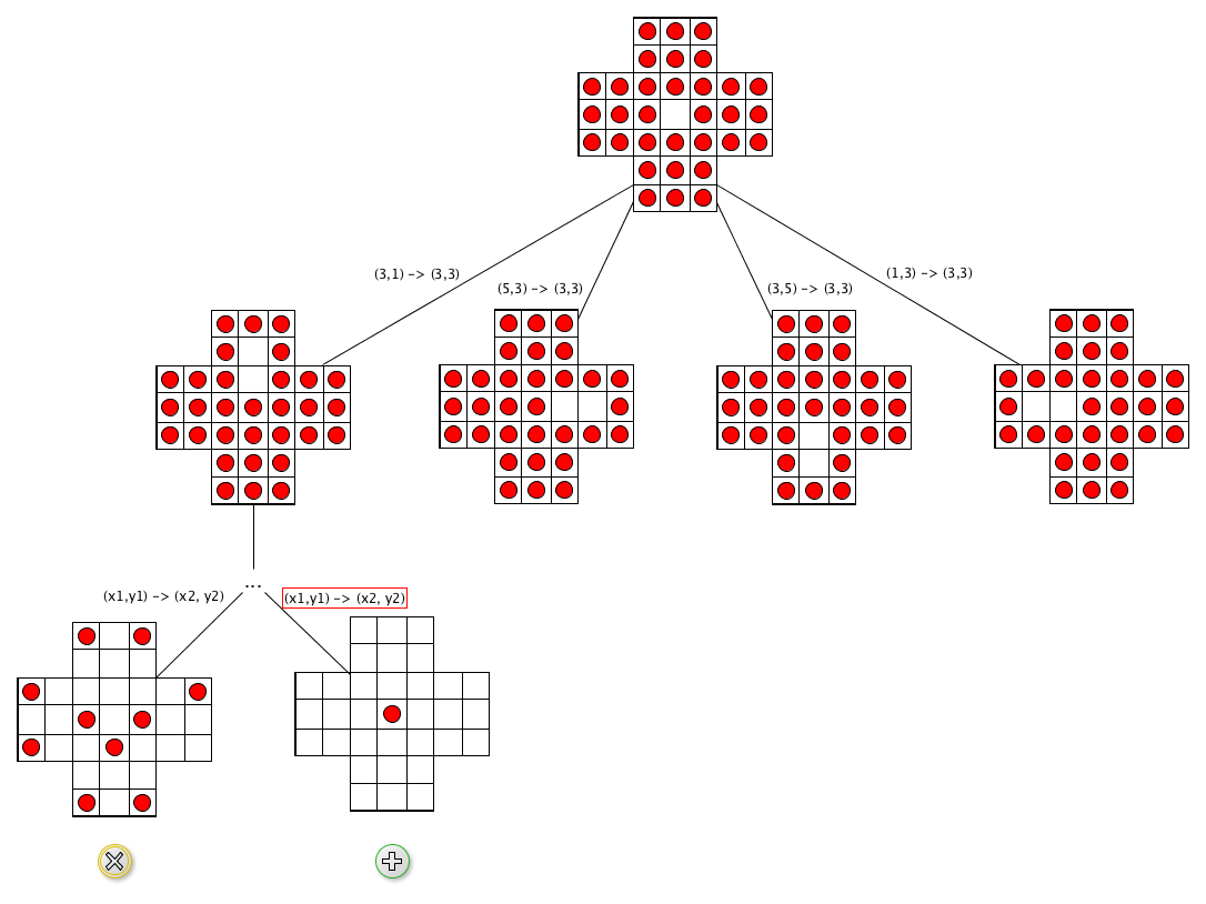
Fig. 50 A sketch of a tree representing the moves a player can make from the initial configuration, which serves as the root of the tree.#
This chapter aims to develop an algorithm for finding a solution to the peg solitaire, considering an alternative board, shown in Fig. 51. This board is the smallest square board on which we can obtain the complement of a given initial configuration of a board by replacing every peg with a hole and vice versa [Bel07]. The advantage of using this board is that the tree of moves’ dimension is relatively small compared with a classic English peg solitaire board. However, it maintains, algorithmically, all the properties of the problem of the more complex one.
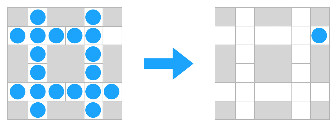
Fig. 51 The complement problem of the peg solitaire, depicted on a 6x6 square board.#
      (1,0)             (4,0)
(0,1) (1,1) (2,1) (3,1) (4,1) (5,1)
      (1,2)             (4,2)
      (1,3)             (4,3)
(0,4) (1,4) (2,4) (3,4) (4,4) (5,4)
      (1,5)             (4,5)
To implement it in Python, we need to find a way for representing all the possible positions of the peg solitaire board in a computationally sound way. To this end, we use a tuple of two elements, depicting x-axis and y-axis values, as representative of a particular position. The collection of all these tuples, shown in Listing 54, represents our board from a purely computational point of view.
 1def create_board():
 2    initial_hole = (5, 1)
 3    holes = set()
 4    holes.add(initial_hole)
 5
 6    pegs = set([
 7        (1, 0), (4, 0),
 8        (0, 1), (1, 1), (2, 1), (3, 1), (4, 1),
 9        (1, 2), (4, 2),
10        (1, 3), (4, 3),
11        (0, 4), (1, 4), (2, 4), (3, 4), (4, 4), (5, 4),
12        (1, 5), (4, 5)
13    ])
14
15    return pegs, holes
According to this organisation, we use two sets for representing a particular status of the board, i.e.:
the set pegs that includes all the pegs available on the board – in the initial status, this set contains all the positions except the final one, i.e.
(5, 1);the set holes that includes all the positions without any peg on the board – in the initial status, this set has just one position, i.e.
(5, 1).
The ancillary function introduced in Listing 55, i.e. create_board(), provides the initial configuration of the solitaire. The result of the execution of this function is a tuple of two elements. In the first position, there is a set of all the pegs at the initial state. In the second position, there is a set of all the available holes at the initial state.
 1from anytree import Node
 2
 3def valid_moves(pegs, holes):
 4    result = list()
 5
 6    for x, y in holes:
 7        if (x-1, y) in pegs and (x-2, y) in pegs:
 8            result.append(Node({"move": (x-2, y), "in": (x, y),
 9                                "remove": (x-1, y)}))
10        if (x+1, y) in pegs and (x+2, y) in pegs:
11            result.append(Node({"move": (x+2, y), "in": (x, y),
12                                "remove": (x+1, y)}))
13        if (x, y-1) in pegs and (x, y-2) in pegs:
14            result.append(Node({"move": (x, y-2), "in": (x, y),
15                                "remove": (x, y-1)}))
16        if (x, y+1) in pegs and (x, y+2) in pegs:
17            result.append(Node({"move": (x, y+2), "in": (x, y),
18                                "remove": (x, y+1)}))
19
20	return result
Another essential task we need to deal with is taking all the possible moves one can do according to the board’s current configuration. The approach used, described in Listing 56 and named valid_moves(pegs, holes), tries to find all the possible moves in the proximity of each hole. In particular, starting from a hole defined by the coordinates (x, y), it looks for a vertical or horizontal sequence of two pegs that creates the condition for performing a valid move.
Each move found is described by a particular small dictionary with the following three keys:
move, which indicates the peg one wants to move;
in, which shows the position where we placed the selected peg after the move (i.e. the hole in consideration);
remove, which indicates the peg that we removed from the board due to the move.
As highlighted in Listing 56, we use the compact constructor for defining dictionaries on-the-fly in Python, i.e. {<key_1>: <value_1>, <key_2>: <value_2>, ...}. For instance, the dictionary my_dict = {"a": 1, "b": 2} can be obtained as well by applying the following operations: my_dict = dict(), my_dict["a"] = 1, my_dict["b"] = 2.
 1def apply_move(node, pegs, holes):
 2    move = node.name
 3    old_pos = move.get("move")
 4    new_pos = move.get("in")
 5    eat_pos = move.get("remove")
 6
 7    pegs.remove(old_pos)
 8    holes.add(old_pos)
 9
10    pegs.add(new_pos)
11    holes.remove(new_pos)
12
13    pegs.remove(eat_pos)
14    holes.add(eat_pos)
15
16def undo_move(node, pegs, holes):
17    move = node.name
18    old_pos = move.get("move")
19    new_pos = move.get("in")
20    eat_pos = move.get("remove")
21
22    pegs.add(old_pos)
23    holes.remove(old_pos)
24
25    pegs.remove(new_pos)
26    holes.add(new_pos)
27
28    pegs.add(eat_pos)
29    holes.remove(eat_pos)
We encapsulate each dictionary defining a move as the name of a tree node. In particular, we create a node using the constructor defined by the package anytree we introduced in the previous chapter. The function in Listing 56 returns a list of all the possible valid moves according to the particular configuration of the board.
We need two additional functions. They take as input a move defined by a tree node and a particular configuration of the board and return the new configuration as if we apply or undo the move, respectively. These functions, i.e. apply_move(node, pegs, holes) and undo_move(node, pegs, holes), are defined in Listing 57.
as part of the material of the course and includes the related test cases.# 1def solve(pegs, holes, last_move):
2 result = None
3
4 if len(pegs) == 1 and (5, 1) in pegs: # leaf-win base case
5 result = last_move
6 else:
7 last_move.children = valid_moves(pegs, holes)
8
9 if len(last_move.children) == 0: # leaf-lose base case
10 undo_move(last_move, pegs, holes) # backtracking
11 else: # recursive step
12 possible_moves = deque(last_move.children)
13
14
15 while result is None and len(possible_moves) > 0:
16 current_move = possible_moves.pop()
17 apply_move(current_move, pegs, holes)
18 result = solve(pegs, holes, current_move)
19
20 if result is None:
21 undo_move(last_move, pegs, holes) # backtracking
22
23 return result
Finally, we need to use a particular comparison operator, i.e. is (and its inverse, is not), which we did not use in the past chapter. This operator checks the identity of the objects instead of the values they may refer to. In particular, <obj1> is <obj2> returns True if the two objects (or two variables referring to two objects) are the same object; otherwise, it returns False. The is not operator works oppositely. It is worth mentioning that checking for the identity of two objects is different from checking for their equality (through the operator ==). In particular, consider the two lists in Listing 59.
1list_one = list()
2list_one.append(1)
3list_one.append(2)
4list_one.append(3)
5
6list_two = list()
7list_two.append(1)
8list_two.append(2)
9list_two.append(3)
The expression list_one == list_two returns True since the lists are equal according to the values they contain. However, the expression list_one is list_two returns False since they are two distinct instances of the Python class list.
We have now all the ingredients for implementing the function for finding a solution of the peg solitaire, according to the backtracking principles introduced at the beginning of this section. Listing 58 presents the final function. For running the function properly, we should initialise the last_move parameter as the root node of the tree of moves built by the function’s execution, e.g. Node("start").
References#
George I. Bell. A Fresh Look at Peg Solitaire. Mathematics Magazine, 80(1):16–28, February 2007. URL: https://www.jstor.org/stable/pdf/27642987.pdf (visited on 2025-10-11), doi:10.1080/0025570X.2007.11953446.
David Silver, Aja Huang, Chris J. Maddison, Arthur Guez, Laurent Sifre, George Van Den Driessche, Julian Schrittwieser, Ioannis Antonoglou, Veda Panneershelvam, Marc Lanctot, Sander Dieleman, Dominik Grewe, John Nham, Nal Kalchbrenner, Ilya Sutskever, Timothy Lillicrap, Madeleine Leach, Koray Kavukcuoglu, Thore Graepel, and Demis Hassabis. Mastering the game of Go with deep neural networks and tree search. Nature, 529(7587):484–489, January 2016. URL: http://web.iitd.ac.in/~sumeet/Silver16.pdf (visited on 2025-10-11), doi:10.1038/nature16961.
David Silver, Julian Schrittwieser, Karen Simonyan, Ioannis Antonoglou, Aja Huang, Arthur Guez, Thomas Hubert, Lucas Baker, Matthew Lai, Adrian Bolton, Yutian Chen, Timothy Lillicrap, Fan Hui, Laurent Sifre, George Van Den Driessche, Thore Graepel, and Demis Hassabis. Mastering the game of Go without human knowledge. Nature, 550(7676):354–359, October 2017. URL: https://www.gwern.net/docs/rl/2017-silver.pdf (visited on 2025-10-11), doi:10.1038/nature24270.