Computability#
This chapter introduces the notion of computability and the computational cost of algorithms. The historic hero presented in these notes is Alan Turing, considered the father of Theoretical Computer Science and Artificial Intelligence. His work on a particular model of computation, known as the Turing machine, had been the primary tool for highlighting the possibilities and the limits of automatic computation and, more in general, the modern electronic computer.
Note
The slides for this chapter are available within the book content.
Historic hero: Alan Turing#
Alan Mathison Turing (shown in Fig. 10) was a computer scientist. His works spanned several disciplines, including mathematics, logic, philosophy, and biology – which is why people have referred to him as a natural philosopher [DC13]. He is considered the father of Theoretical Computer Science and Artificial Intelligence due to its frontier contributions that provided his theoretical machine named after him [Tur37][1]. Besides, his studies on the relationship between electronic computers and intelligence [Tur50] brought him to define the thought experiment known as the Turing test.
He was one of the key figures behind the decryption of Enigma, the cypher machine used by Nazi Germany for protecting communications[2]. Also, his studies do not focus only on Computer Science topics. They include essential works in Biology. In particular, he described how natural patterns (e.g. stripes, spots and spirals) might spontaneously arise out of a uniform state [Tur52].
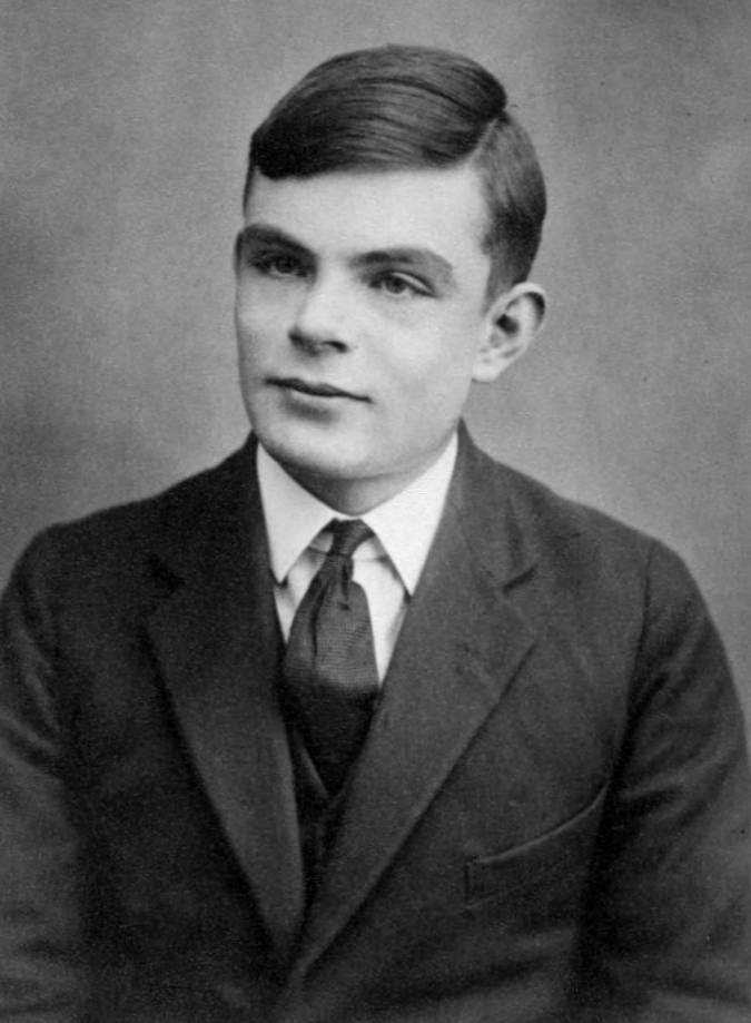
Fig. 10 Picture of Alan Turing taken in 1927. Source: Wikipedia.#
The Turing machine#
In 1936, Turing developed his machine to answer an important issue related to Hilbert’s decision problem, which asks about the possibility of creating an algorithm for deciding if a first-order logic formula is universally valid or not. Alonzo Church also analysed the problem simultaneously by addressing it from a totally different (but pragmatically equivalent) perspective than Turing’s approach. The machine proposed by Turing was only theoretical. Indeed, he did not build it physically. Recently, several people provided physical prototypes of Turing’s idea, such as the one shown in Fig. 11.
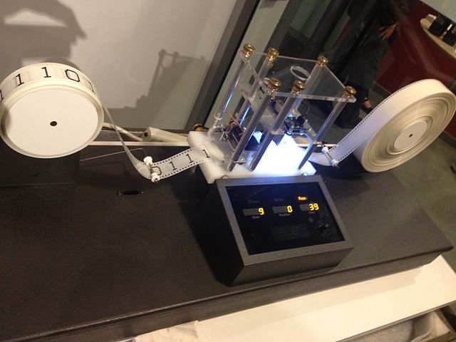
Fig. 11 A physical implementation of a Turing machine with a finite tape. Picture by GabrielF, source: Wikimedia Commons.#
The Turing machine can simulate any algorithm using a pretty simple set of tools. It is composed of an infinite memory tape containing cells. Each cell can have a symbol (i.e. either 0 or 1, where 0 is the blank symbol, assigned to all the cells in advance) that can be read and written by the head of the machine. The state of the machine at a specific time is recorded. The machine specifies the possible actions to perform in a finite table of instructions. Each instruction in the table says what to do: write a new symbol, move the head either left or right, go to a new state. The machine selects a particular instruction according to the current state and the current symbol under the head. An initial state and zero or more final states are provided to define where to start and end the process.
For instance, in Table 2, there is a representation of a table of instructions for a simple Turing machine, where: A is the initial state, and there are no final states. Each row in the table represents a particular instruction. For instance, the first row says that being in A, if the head reads 0 or 1 on the tape, then 1 is written down, the head is moved one cell to the right, and the new state of the machine becomes B.
Current state |
Tape symbol |
Write symbol |
Move head |
Next state |
|---|---|---|---|---|
A |
0 or 1 |
1 |
right |
B |
B |
0 or 1 |
0 |
right |
A |
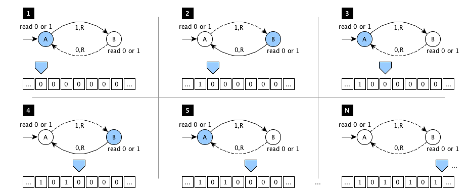
Fig. 12 A graphical representation of the execution of the Turing machine implementing the rules introduced in Table 2. In the various figures, the blue polygon represents the head of the machine, positioned in a specific cell of the tape. The blue circle represents the current state, while the solid arrow depicts the next state, reached once the machine writes the symbol in the label of the solid arrow in the cell pointed by the head. Finally, the machine moves the head in the direction indicated on the label (where R stands for right).#
Also, we can represent the table of instructions of a Turing machine graphically. For example, we can use labelled circles for representing states. Also, we can use arrows pointing to the next states when a particular symbol is read on the tape. The machine writes the symbol indicated in the label of an arrow when such an arrow is followed. Similarly, the head of the machine is moved according to the direction (i.e. left or right) indicated in the arrow’s label. For instance, in Fig. 12, it is shown the execution of the Turing machine related to the table of instructions introduced in Table 2. In particular, this Turing machine has the characteristic of running forever – it will never stop its execution – since it writes several 1s separated by 0s indefinitely. Thus, practically speaking, this Turing machine demonstrates that it is possible to develop algorithms that run forever without ever ending their execution.
While the Turing machine is quite a simple tool, it enables one to model computation in the broad sense. While Turing has not proposed it as a sketch for developing electronic computers, its theoretical properties also apply to real computing machines. In particular, an electronic computer can compute anything that a Turing machine can compute. This property has been used to prove the intrinsic limitations on the power of mechanical computation.
People have developed several tools to simulate a Turing machine. The Turing Machine Visualization is one such tool, mainly designed for academic purposes. It is a simple web application that allows one to define all the components of a Turing machine through straightforward language. Once defined the initial state, initialised the tape with 0s, and defined the table of instructions, one can watch the way the machine runs. In particular, each step of the execution is shown graphically.
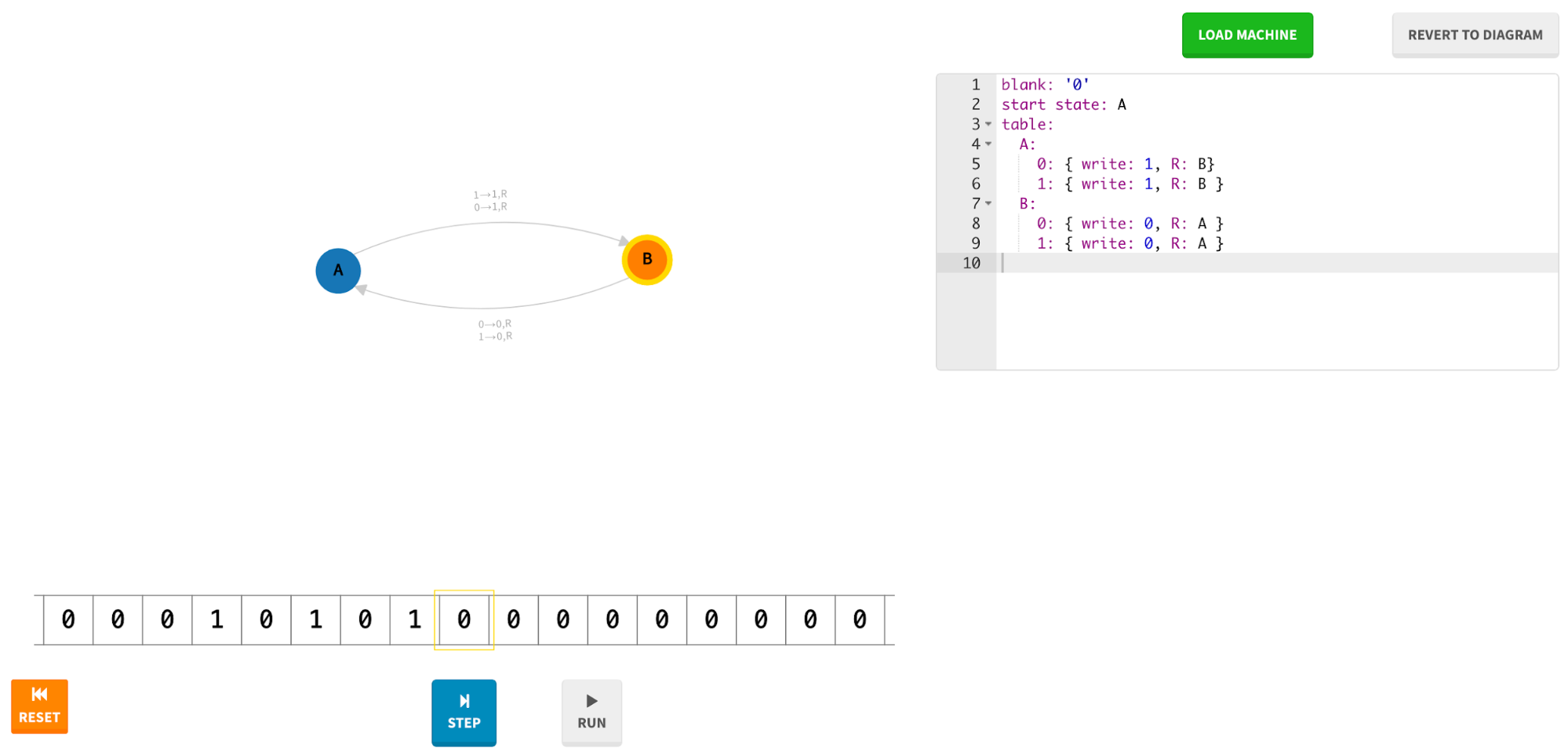
Fig. 13 A screenshot of the Web application Turing Machine Visualization.#
The various variables can be specified using the template in Listing 8.
1blank: '0'
2start state: <start state>
3table:
4  <state>:
5    <tape symbol>: { write: <symbol>, <R or L move>: <next state> }
6    <end state>:
Where blank says how to initialise the tape, the table is composed by one or more <state>s, one of which is used as <start-state>, and one or more (optional) <end state>s can be specified as well – they is recognisable since no operations have been defined on them. Following the template above, the Turing machine described in Table 2 is defined in Listing 9.
1blank: '0'
2start state: A
3table:
4  A:
5    0: { write: 1, R: B }
6    1: { write: 1, R: B }
7  B:
8    0: { write: 0, R: A }
9    1: { write: 0, R: A }
Fig. 13 shows the Turing machine implemented by these instructions. Three distinct areas realise the whole visualisation of the machine. First, a text box contains the rules written according to the template mentioned above. Second, a graph represents the table of instructions of the machine. Finally, a sequence of cells represents the tape, where a yellow box highlights the head of the machine.
The computational cost of an algorithm#
In the previous lecture, we have defined what an algorithm is and the relation that exists between algorithms and computers. In the previous section, we have seen how a simple machine, which implements an algorithm using a specific language, can compute indefinitely. On the other hand, other machines could compute a result in a reasonable finite time. And, even algorithms can spend an exaggerated time (if still limited) to return a result. Thus, it can be helpful to know how much time indicatively an algorithm needs to produce a result.
This issue is the core topic of one of the essential branches of the theory of computation, i.e. the computational complexity theory. The research in this field aims at classifying computational problems. A computational problem is a problem that can be solved algorithmically by a computer. Each computational problem, thus, can be classified according to a hierarchy of categories. Each category expresses the difficulty in solving such a problem.
An important subfield of computational complexity theory is the analysis of algorithms. Analysing an algorithm means understanding the amount of time, storage and other resources needed to execute such an algorithm. In particular, usually, this analysis focuses on finding a specific mathematical function that relates the input of an algorithm with the number of instructions that are run to return the final result from that input. The lesser the instructions to execute, the more efficient the algorithm will be.
It is worth mentioning that the measure provided by such function is not precise since it is only an upper bound of the actual performance. However, it is enough to indicate the time needed to execute a particular algorithm on a specific input.
We do not want to introduce all the theoretical principles and the proper mathematical tools for addressing such analysis since it is out of the scope of the course[3]. The message to reinforce is that the strategy used to develop an algorithm affects, positively or negatively, its efficiency. It is possible to create two different algorithms addressing the same computational problem that take different times for returning the result.
Can we compute everything?#
After reading all the material introduced in the previous sections, the main question one could ask is: can we use algorithms for computing whatever we want? In other words: there exists a limitation on what we can compute? Or, even: is it possible to define a computational problem that any algorithm cannot solve?
Usually, computer scientists and mathematicians use reductio ad absurdum to demonstrate that something cannot exist. Reduction ad absurdum aims at coming to a paradoxical and self-contradictory situation, such as the fact that the existence of an algorithm contradicts its existence itself. This kind of argument seeks to establish a contention by deriving an absurdity from its denial, thus arguing that a thesis must be accepted because its rejection would be untenable [noa] and, eventually, generates paradoxes.
Paradoxes have mainly been used in logic in the past. While they are funny stories to tell for teaching, they are also powerful tools for showing limits or constraints of a particular formal aspect of a field or situation. For instance, one of the most famous paradoxes in mathematics is the Russell paradox, discovered by Bertrand Russell in 1901. It was one of the most important discoveries of the beginning of the twentieth century. It has proved that the current set theory proposed by Georg Cantor, and used as the foundation for Gottlob Frege’s work on the definition of the fundamental laws of arithmetic, led to a contradiction. Thus, it invalidated the set theory and the work done by Frege – that was in print when Russell communicated his discovery to him. A variation to that paradox could be formulated as follows.
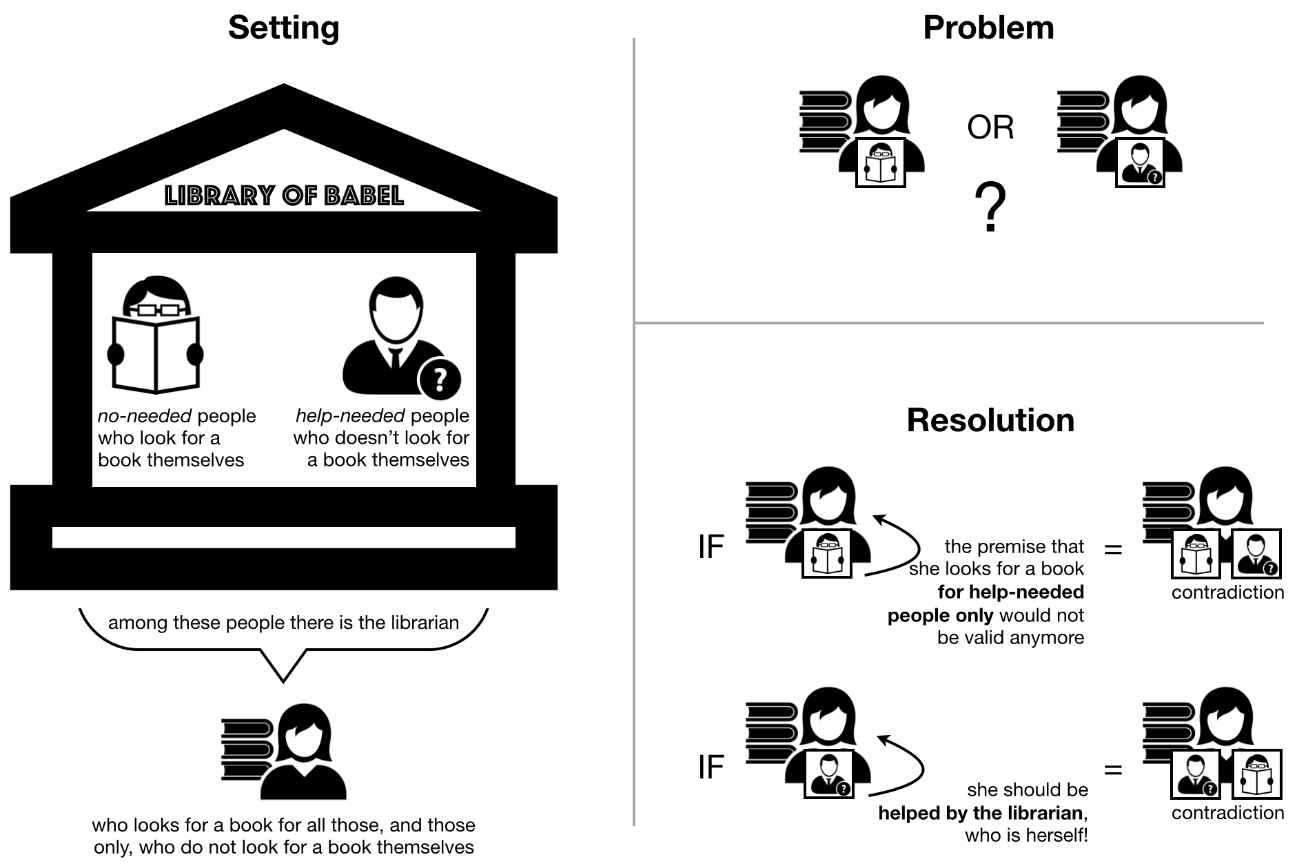
Fig. 14 A graphical representation of the librarian paradox, which is a puzzle derived from Russell’s paradox.#
Librarian paradox: In the Library of Babel, there are people of two different kinds. The first kind of people – named no-needed – are those who look for a book themselves. The other type of people – named help-needed – are those who do not look for a book themselves, and thus they need help doing it. One of the people in the library is the librarian. The librarian looks for books for all those, and those only, who do not look for books themselves (i.e. the help-needed people). The question is: who looks for books to the librarian?
Resolution: On the one hand, if the librarian is a no-needed person (who looks for a book herself), then the premise that the librarian should look for books only for help-needed people would not be valid anymore. Thus, if she is a no-needed person, she is a help-needed person, which is a contradiction. On the other hand, if the librarian is a help-needed person – and, as such, she is not able to look for books herself – she should be helped by the librarian, who is herself! Therefore, if she is a help-needed person, she is also a no-needed person – which is another contradiction.
One of the most attractive problems that computer scientists studied in the past was part of the 23 open mathematical problems David Hilbert proposed in 1900. It is known as the halting problem. This problem was meant to prove whether a particular algorithm will terminate its execution at some point or it will run forever. In the previous lecture, we have developed our first algorithm. We have defined it to always return a value as an outcome, which confirms that we can create algorithms that terminate. Besides, as demonstrated in Section The Turing machine, we have also shown an algorithm (implemented by the Turing machine summarised in Fig. 12) that runs indefinitely. Thus, an approach that systematically us to discover whether an algorithm will terminate or not is a great tool to have. Indeed, it would enable the identification of computationally-ill algorithms.
Alan Turing created his machine for answering such a question: to prove if we can develop a Turing machine (i.e. an algorithm) that can decide whether another machine will terminate its execution or not. An approximation of the solution provided by Turing is introduced as follows. It uses a reductio ad absurdum argument, which is very close to the one presented in Fig. 14 for resolving the librarian paradox.
Suppose we have the algorithm “does it halt”, as shown in Fig. 15, which returns yes if the execution of a particular input algorithm terminates, while it returns no otherwise. This algorithm is just hypothetical. We are supposing that we can develop it somehow, without providing it in any particular programming language.
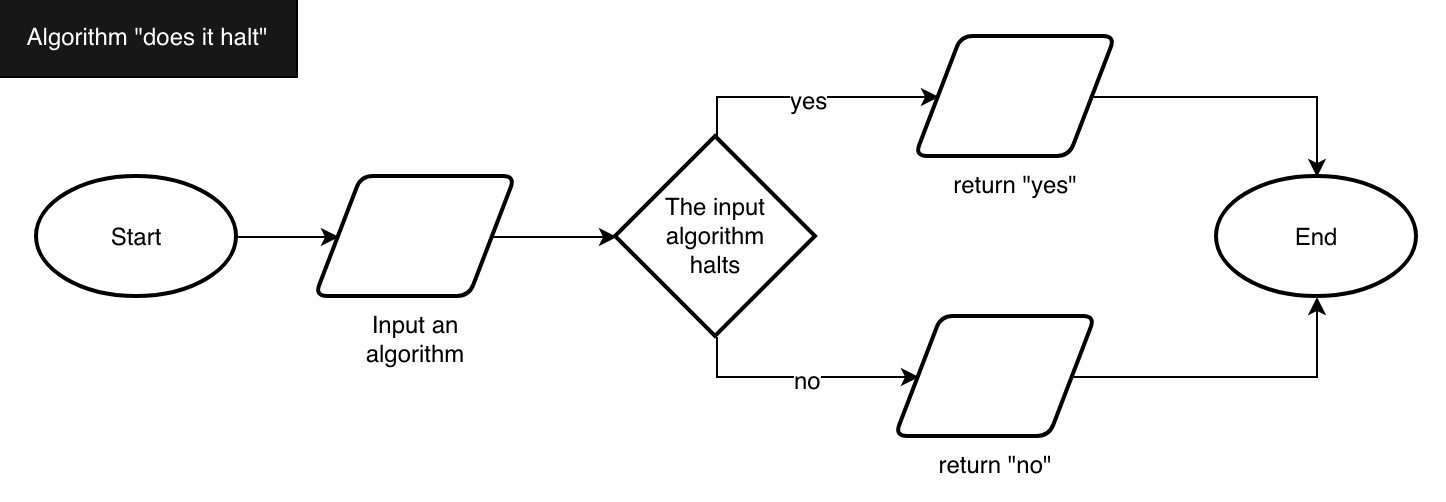
Fig. 15 The flowchart of the “does it halt” algorithm that returns “yes” if the input algorithm halts and returns “no” otherwise.#
Then we reuse the “does it halt” algorithm for developing a new algorithm, shown in the flowchart in Fig. 16. In particular, this new algorithm takes another algorithm as input and, if the input algorithm stops, it runs forever. Otherwise, if the input algorithm does not terminate, then it stops. Please note that we know how to implement the various steps of this new algorithm. Indeed, checking whether the input algorithm can terminate or not is provided by the algorithm “does it halt” introduced in Fig. 15. Moreover, the “Run forever” process operation is implementable by a machine since we have already developed a Turing machine (presented in Section The Turing machine) that does so.
Now, the question is: what happens if we try to execute the algorithm described in Fig. 16 by passing itself as input? We have two possible situations:
If the algorithm “does it halt” says that our algorithm depicted in Fig. 16 stops, then our algorithm runs forever;
if the algorithm “does it halt” says that our algorithm shown in Fig. 16 does not stop, then our algorithm stops.
Hence, whatever is the behaviour of the algorithm introduced in Fig. 16, it always generates a contradiction. Consequently, the main algorithm used in the decision widget, i.e. the algorithm “does it halt”, cannot be developed. Thus, the answer to the halting problem mentioned before is that the algorithm that checks if another one stops cannot exist.
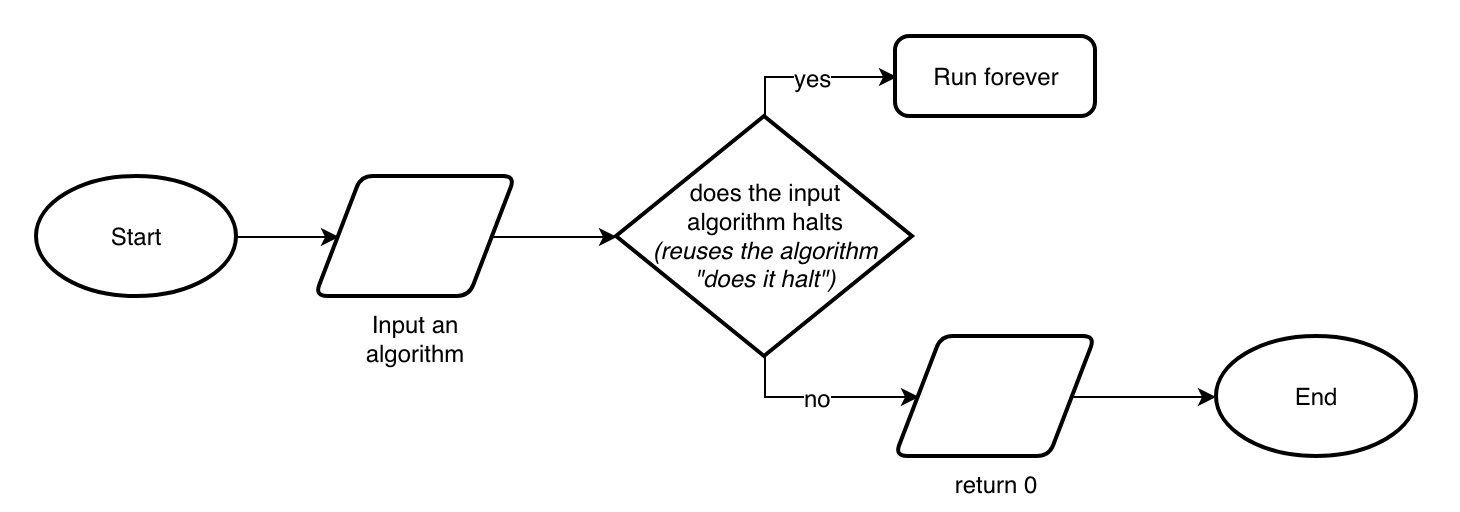
Fig. 16 The flowchart of an algorithm that runs forever if the execution of another algorithm specified as input (and checked by using the algorithm presented in Fig. 15) stops, and it stops otherwise. Please note that the process step “Run forever” of the flowchart algorithm can be easily developed. In fact, in Section The Turing machine, we have shown a simple Turing machine that implements such behaviour.#
This result had a disruptive effect on the perception of computational abilities at large. In practice, Turing’s machines and their analyses posed clear limits to what we can compute. Moreover, they enabled him to explicitly state that specific computational problems cannot be solved, such as the halting problem mentioned in this section.
References#
Reductio ad Absurdum. URL: http://www.iep.utm.edu/reductio/.
Gordana Dodig-Crnkovic. Alan Turing’s Legacy: Info-computational Philosophy of Nature. In Gordana Dodig-Crnkovic and Raffaela Giovagnoli, editors, Computing Nature, volume 7, pages 115–123. Springer Berlin Heidelberg, Berlin, Heidelberg, 2013. URL: https://arxiv.org/ftp/arxiv/papers/1207/1207.1033.pdf (visited on 2025-09-13), doi:10.1007/978-3-642-37225-4_6.
Alan Mathison Turing. On Computable Numbers, with an Application to the Entscheidungsproblem. Proceedings of the London Mathematical Society, s2-42(1):230–265, 1937. URL: http://doi.wiley.com/10.1112/plms/s2-42.1.230 (visited on 2025-09-13), doi:10.1112/plms/s2-42.1.230.
Alan Mathison Turing. Computing Machinery and Intelligence. Mind, LIX(236):433–460, October 1950. URL: https://academic.oup.com/mind/article/LIX/236/433/986238 (visited on 2025-09-13), doi:10.1093/mind/LIX.236.433.
Alan Mathison Turing. The chemical basis of morphogenesis. Philosophical Transactions of the Royal Society of London. Series B, Biological Sciences, 237(641):37–72, August 1952. URL: https://royalsocietypublishing.org/doi/10.1098/rstb.1952.0012 (visited on 2025-09-13), doi:10.1098/rstb.1952.0012.
Stephen Wolfram. Statistical mechanics of cellular automata. Reviews of Modern Physics, 55(3):601–644, July 1983. URL: https://link.aps.org/doi/10.1103/RevModPhys.55.601 (visited on 2025-09-13), doi:10.1103/RevModPhys.55.601.
Stephen Wolfram. A new kind of science. Wolfram Media, Champaign, IL, 2002. ISBN 978-1-57955-008-0. URL: https://www.wolframscience.com/nks/p169--introduction/.