Programming Languages

This chapter provides a general introduction to programming languages and then focuses on a particular language: Python. The historic hero introduced in these notes is Grace Hopper. She was the first programmer of the Harvard Mark I computer. She was responsible for the development of some of the first programming languages.

Note

The slides for this chapter are available within the book content.

Historic hero: Grace Hopper

Grace Brewster Murray Hopper (depicted in Fig. 17 was a computer scientist. She was the first programmer of the Harvard Mark I, i.e. a general-purpose electromechanical computer. The Harvard Mark I was used during the Second World War, fully-inspired by Babbage’s Analytical Engine. She pushed for the need of having machine-independent programming languages. This idea brought her in the development of COBOL, one of the first high-level programming languages, which is still used today for some applications.

COBOL (i.e. the common business-oriented language) is a programming language designed for business use. It brings a quite extensive use of English terms for describing the operations of a program. For the very first time, the idea of adopting English for commands made the programming language a bit more verbose and more readable and even self-documenting. Just for making an example, in today’s languages if we want to compare if the value assigned to a variable x is greater than the one assigned to another variable y we should use x > y. In COBOL, the same comparison is made with the following instruction: x IS GREATER THAN y.

Fig. 17 Portrait of Grace Hopper. Picture by James S. Davis, source: Wikipedia.

A brief history of programming languages

After the Second World War, people have developed several programming languages according to several design principles and intended usage in terms of the computational problems to be solved. While all of them, in principle, make it possible to develop solutions for any solvable computational problem, some of them are more suited for a specific domain than others. For instance, COBOL has been developed for business applications, while FORTRAN was designed to deal with scientific computing.

While an extensive analysis of all the programming languages is out of the scope of the topics of this book, it is worth mentioning, at least graphically, a timeline of their evolution, shown in Fig. 18. As highlighted in the timeline, we will introduce and use a particular programming language in this course, i.e. Python, according to its third version released in 2006.

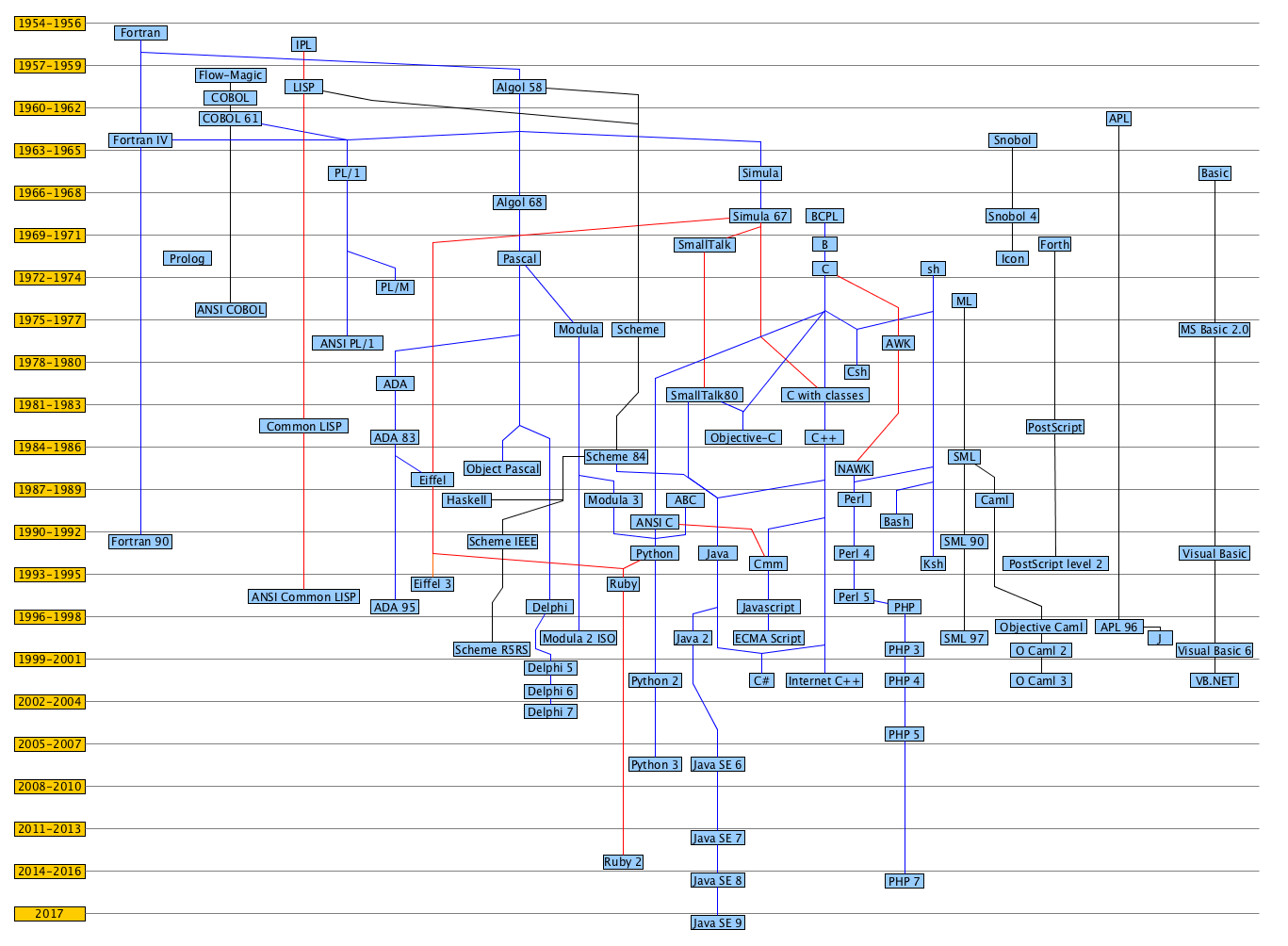
Fig. 18 A graphic timeline summary of some of the main programming languages from 1954 to 2017. The different line colour is used only for readability reasons, and it does not have any particular meaning.

Python

Python is a high-level programming language for general-purpose programming. It is currently one of the most used languages for programming on the Web for Data Science and Natural Language Processing tasks. The good thing about Python is that it is one of the most simple languages for starting to learn how to program and create software.

In this course, we will use Python in its latest version, i.e. Python 3. Luckily, there are a lot of resources freely available online for learning this language from scratch, such as:

• the introductory book Dive into Python 3 [Pil09];

• the official documentation of the language;

• an online platform for playing with Python 3 without installing any software on your computer;

• an interactive online course for learning Python from scratch;

• a book introducing all the basic Python features, which is particularly suited for Digital Humanities [Tag18];

• another book entirely dedicated to problem solving and algorithms developed in Python [MR11];

• a digital book that contains an introduction to Python for the Humanities.

The goal of this chapter is to develop our first algorithm in Python. The algorithm we produce is the one we have introduced in Chapter Algorithms, that can be described informally by the following natural language text:

Consider three different strings as input, i.e. two words and a bibliographic entry of a published paper. The algorithm must return the number 2 if the bibliographic entry contains both words; the number 1 if the bibliographic entry contains only one word; the number 0 otherwise.

First incomplete version, in Python

In Python, we can create a new algorithm by implementing a new function. We can introduce a function using the keyword def (which stands for define). The keyword def must be followed by a name (e.g. the name of the algorithm) and a comma-separated list of input parameters between round brackets. For instance, def contains_word(first_word, second_word, bib_entry) defines the function contains_word, which takes three parameters as input​.

Each function definition is followed by “:” and all the instructions to execute must be specified in the following lines, as an indented block (preferably using four spaces), as illustrated in Listing 10. The name of a function and its parameters cannot contain space characters and must always start with a letter – e.g. this_is_my_parameter is correct, while 1_parameter is not.

Listing 10 The definition of an algorithm, with its input parameter, and some dots that identify where to put the instruction of such algorithm – one per line, indented of 4 space characters.

​def contains_word(first_word, second_word, bib_entry):
    ...
    ...
    ...

In this first version of the algorithm, we would like to introduce only some basic constructs of Python. To this end, we provide only a partial solution in this subsection, which we finalise in the following subsections, following the same strategy used in Chapter Algorithms. In particular, we want to say that if the bibliographic entry contains the first input word, the number 1 is returned; otherwise, a 0 is returned. Listing 11 shows this incomplete version of the algorithm in Python.

Listing 11 An incomplete version of the algorithm that is used to introduce some basic constructs of Python.

def contains_word(first_word, second_word, bib_entry):
    if first_word in bib_entry:
        return 1
    else:
        return 0

In this incomplete version, there are already specified some important constructs of Python. The first one is the if-else conditional block. This kind of block allows one to execute a particular instruction if a condition is true (the if statement). Otherwise, if the condition specified is false, an alternative set of instructions is executed instead (the else statement). We can avoid specifying the else clause if no alternative set of instructions is needed. The instructions to perform in one case or the other are within indented sub-blocks (again, four additional spaces). As already introduced in Listing 11, every time we have to add a new block of instructions, we need to use ​: after the statement of interest, as shown in Listing 12.

Listing 12 The generic structure of an if-else conditional block.

​if <condition>:
    ...
    ...
else:
    ...
    ...

The condition specified in the if statement shown in Listing 11 allows one to check if a certain string is contained in another one using the command “in”. In particular, <string1> in <string2> would be true if <string2> contains <string1>. As anticipated in the previous chapters, a string is a particular type of value composed of a sequence of characters and defined by using quotes. For instance, "Peroni", "Osborne", and ​"Peroni, S., Osborne, F., Di Iorio, A., Nuzzolese, A. G., Poggi, F., Vitali, F., Motta, E. (2017). Research Articles in Simplified HTML: a Web-first format for HTML-based scholarly articles. PeerJ Computer Science 3: e132. e2513. DOI: https://doi.org/10.7717/peerj-cs.132" are all strings.

Note that and are just placeholders for strings: we can use either strings, e.g. "Peroni" in "Peroni beer", or variables referring to strings, as shown in Listing 11. A variable is a symbolic name that contains some information referred to as a value (e.g. first_word). For instance, any input value is, in fact, a particular kind of variable. As defined previously, all the input parameters of the algorithm are expected to refer to strings.

The last construct of the partial algorithm introduced in this subsection is the return statement. It is defined by specifying the token return followed by the value (or the variable containing a value) that must be returned. The execution of a return statement concludes the algorithm execution. Thus, all the instructions that follow that statement are not processed anymore. In the example in Listing 11, two different numbers are returned, depending on the execution of a particular branch of the if-else block. In particular, the algorithm returns a 1 if the condition of the if statement is true, while it returns a 0 otherwise. Python permits to write any number as it is – e.g. ​42 and -42 for positive/negative integers, 1.625 and -1.625 for positive/negative decimals. Note that strings and numbers are distinct kinds of objects – e.g. the string "42" and the number 42 (without the quotes) do not define the same value.

Complex boolean statements

The original text of the algorithm, introduced at the beginning of Section Python, needs to condition to be true for returning a 2. Indeed, the bibliographic entry must contain both words. This can be defined using a hierarchy of if-else blocks in Python, as shown in Listing 13.

Listing 13 A hierarchy of if-else blocks for describing the three possible return values of the algorithm.

​if first_word in bib_entry:
    if second_word in bib_entry:
        return 2
    else:
        return 1
else:
    if second_word in bib_entry:
        if first_word in bib_entry:
            return 2
        else:
            return 1
    else:
        return 0

However, the readability of the previous example is rather difficult since it repeats several times the same conditions, even if they have been specified in a different order. Thus, Python makes available some operations for assessing compositions of multiple boolean values and for deriving boolean values from number and string comparisons. A boolean value (or, directly, boolean)[1] can be only one of two distinct and disjoint values, True and False. For instance, the condition first_word in bib_entry returns a particular boolean: True if the bibliographic entry contains the word, False otherwise. We use boolean values in algorithms (and in any programming language) to organise conditional block execution flow.

Sometimes it is useful to combine somehow two distinct boolean values to simplify the conditional blocks’ organisation. This can be done by using specific operators that apply to one (<operator> <B1>) or two boolean values (<B1> <operator> <B2>), and return a new boolean value. These operators are called logical not (​not in Python, which applies to one boolean value only), *logical and *(​and, between two boolean values), and logical or (​or, between two boolean values). They are logical operators since they derive from the logic Boole proposed in his works on Boolean algebra. Table 3 summarises their use and shows the truth table of the application of such operators. In particular, given two boolean input values, B1 and B2, the table shows the result of all their possible combinations according to the specific operator. Thus, in the example in Listing 13, we could return a 2 if the bibliographic reference contains both the strings, expressing this constraint in one condition only, i.e. first_word in bib_entry and second_word in bib_entry.

Table 3 The truth table of all the boolean operations.

B1	B2	not B1	B1 and B2	B1 or B2
True	True	False	True	True
True	False	False	False	True
False	True	True	False	True
False	False	True	False	False

Round brackets can be used for grouping boolean operations, e.g. (True and False) or False applies the and operation first, and the result is used as the first value of the or operation – given False as a result. If there are no brackets, the application order proceeds as follows. First, one must execute all the not operations. Then, one must perform all the and operations. Finally, one must assess the remaining or operations. For instance, ​True and not False or False returns True since it is interpreted as (True and (not False)) or False.

Table 4 The truth table of all string comparisons.

S1	S2	S1 < S2	S1 <= S2	S1 > S2	S1 >= S2	S1 == S2	S1 != S2	S1 in S2	S1 not in S2
"Alice"	"Bob"	True	True	False	False	False	True	False	True
"Alice"	"Alice"	False	True	False	True	True	False	True	False

In addition to the aforementioned boolean operations, it is also possible to use string comparisons for obtaining boolean values. Table 4 shows all the comparisons that one can apply on two strings, i.e. <S1> <operator> <S2>. In this case, the operators are those typically used numerical comparison, i.e.:

• ​<, less than;

• ​<=, less than or equal to;

• ​>, greater than;

• ​>= greater than or equal to;

• ​==, equal to;

• ​!=, different from;

• ​​in, included in;

• ​not in, not included in.

In the case of strings, a string S1 is less than another string S2 if the former precedes the latter according to a pure alphabetic order. Of course, Python uses the alphabetic order for assessing when a string is greater than another one.

Note that we can use similar operators (excluding in) for comparing numbers, as shown in Table 5. In this case, the standard mathematical numeric comparisons hold.

Table 5 The truth table of all the arithmetic comparisons.

N1	N2	N1 < N2	N1 <= N2	N1 > N2	N1 >= N2	N1 == N2	N1 != N2
3	4	True	True	False	False	False	True
4	4	False	True	False	True	True	False

Thus, we can reuse these boolean operations to rewrite the if-else blocks shown in Listing 13 more understandably. Finally, Listing 14 shows the result.

Listing 14 A hierarchy of if-else blocks shown in Listing 4 rewritten according to the boolean operations presented in this section.

​if first_word in bib_entry and second_word in bib_entry:
    return 2
else:
    if first_word in bib_entry or second_word in bib_entry:
        return 1
    else:
        return 0

Conditional statements with multiple branches

While in the previous subsections we have improved the readability of the if-else blocks, Python allows us to do even better. First of all, in the two if statements in Listing 14, we ask Python to evaluate the same sub-conditions (i.e. first_word in bib_entry and second_word in bib_entry) twice. This can be easily avoided by defining new variables. A variable is defined by specifying its name (without spaces), followed by an = and the value to associate to it, i.e. <variable_name> = <variable_value>. The value can be specified directly (e.g. a number) or indirectly by using other variables or even complex operations.

In our example, we could create two variables, called contains_first_word and contains_second_word, assigned to the boolean returned by the string comparisons mentioned above, i.e. first_word in bib_entry and second_word in bib_entry, respectively. In that way, we can reuse such variables in the two if statements, as shown in Listing 15.

Listing 15 The if-else blocks introduced in Listing 14 where the conditions in if statements are specified using two variables.

​if contains_first_word and contains_second_word:
    return 2
else:
    if contains_first_word or contains_second_word:
        return 1
    else:
        return 0

We can improve further the readability of the code by collapsing occurrences of else statements when these contain an if statement. In this case, both the else-if pair can be safely replaced by an elif (i.e. else if) statement, which specifies the same condition used in the if statement. Thus, the code in Listing 15 can be rewritten, as shown in Listing 16.

Listing 16 The if-else blocks introduced in Listing 6 collapsed using an elif statement.

if contains_first_word and contains_second_word:
    return 2
elif contains_first_word or contains_second_word:
    return 1
else:
    return 0

Final algorithm

In this chapter, we have seen some initial constructs that Python makes available for developing an algorithm. In particular, we have introduced how to define a function with input parameters, variables, conditional statements (i.e. if, elif, and else), string, numeric, and boolean values, boolean operations and string and numeric comparisons. All these constructs enabled us to define our algorithm, which is finally introduced in Listing 17.

Listing 17 The final algorithm developed.

def contains_word(first_word, second_word, bib_entry):
    contains_first_word = first_word in bib_entry
    contains_second_word = second_word in bib_entry


    if contains_first_word and contains_second_word:
        return 2
    elif contains_first_word or contains_second_word:
        return 1
    else:
        return 0

It is worth mentioning that the algorithm proposed initially in Chapter Algorithms as a flowchart does not map with the one presented in Listing 17. This misalignment has been done to explicitly show that it is entirely possible to develop two different algorithms for addressing the same computational problem.

As a final note, and in addition to using the Python interpreter installed on your machine (in any), several Web applications have been developed to test your Python code. Often, they show which kinds of objects Python creates when running. One of these tools, i.e. Python Tutor, is very helpful for people approaching Python for the first time. Indeed, it allows one to see what happens as the (electronic) computer runs each line of code.

Test-driven development

Different development strategies can be adopted when one wants to understand whether the piece of software he/she has developed is correct or not – i.e. if it is returning the expected result. One of the most used and practical methods used by programmers is the Test-Driven Development (or TDD) [Bec03], summarised in Fig. 19.

In practice, when one has a computational problem to solve, and he/she needs to develop a piece of software to address it, the first thing to develop is a test to check if the software that eventually will be developed behaves correctly (i.e. returns the correct result) or not. Usually, such a test is software that must be designed to test the correctness of another software.

Writing a test before starting to develop software allows one to focus on the problem one has to solve and on the requirements of the software from the very beginning. This approach is also practical when one decides to extend an existing software. In this case, first, one has to develop the test for assessing the correctness of such a new extension. Second, one needs to write the extension and check if the extended software passes the new test.

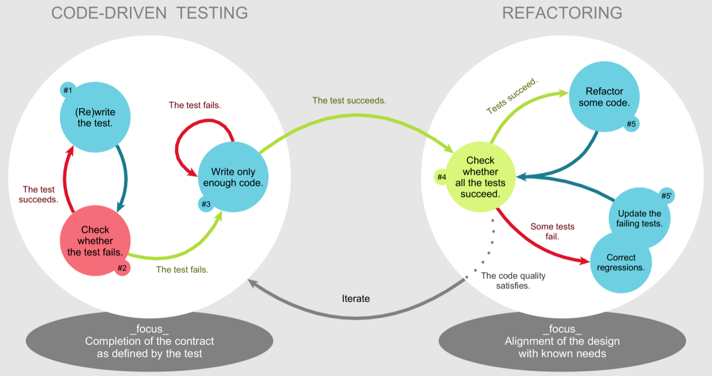
Fig. 19 A diagram summarising the steps of the test-driven development approach. Picture by Xarawn, source: Wikipedia.

1. Write a new test – once understood the computational problem to solve and the related requirements, a new test is written and then added to a collection of previously developed tests.

2. Run all the tests – we run all the tests available in the collection mentioned above. If the new test fails, there is no code available that addresses the particular computational problem described by the test. Thus, the test fails in the first iteration of the test-driven development since no code has been developed yet.

3. Write the new code – in this step, we develop a new code to pass the test just added to the collection.

4. Run all the tests again – in this passage, one checks if the addition of such new code developed to address the new test has not broken the other features already designed and tested by all the other tests available in the collection (in any). If any test fails, the new code must be corrected until all the tests are passed successfully.

5. Refactor the code – after several iterations of the process, the code grows naturally, and it may be necessary to refactor as to clean the code as much as possibleto guarantee its readability and maintainability in the long term. As a suggestion, every refactoring action should be checked by re-run all the tests available to be sure that a modification to the code does not break its correctness.

Following this approach to development is very useful when one has to implement a particular algorithm in Python. It enables one to check its correctness according to different kinds of input that can be used to run the algorithm itself. Listing 18 shows a plausible test to verify the accuracy of the algorithm introduced in this chapter.

Listing 18 The test function developed for testing the contains_word code, introduced in Listing 17.

def test_contains_word(first_word, second_word, bib_entry, expected):
    result = contains_word(first_word, second_word, bib_entry)
    if expected == result:
        return True
    else:
        return False

It is possible to use such a test function to test the contains_word code with different kinds of input values and related expected results. For instance, Listing 19 shows the test code, the algorithm’s code presented in this chapter, and some checks done by running the test code (and thus the algorithm itself) with different input values. Finally, the result of the various inspections is printed on screen by using the Python function print().

Listing 19 The test code, the algorithm implementation in Python, and three distinct runs of the test with different configurations and expected results. The source code of this listing is available as part of the material of the course.

# Test case for the algorithm
def test_contains_word(first_word, second_word, bib_entry, expected):
    result = contains_word(first_word, second_word, bib_entry)
    if expected == result:
        return True
    else:
        return False

# Code of the algorithm
def contains_word(first_word, second_word, bib_entry):
    if first_word in bib_entry and second_word in bib_entry:
        return 2
    elif first_word in bib_entry or second_word in bib_entry:
        return 1
    else:
        return 0

# Three different test runs
print(test_contains_word("Shotton", "Open",
    "Shotton, D. (2013). Open Citations. Nature, 502: 295–297. doi:10.1038/502295a", 2))
print(test_contains_word("Citations", "Science",
    "Shotton, D. (2013). Open Citations. Nature, 502: 295–297. doi:10.1038/502295a", 1))
print(test_contains_word("References", "1983",
    "Shotton, D. (2013). Open Citations. Nature, 502: 295–297. doi:10.1038/502295a", 0))

The proposed development approach could seem bland at first sight. However, programmers regularly adopt it to think carefully about the requirements of a particular code to develop and avoid the introduction of bugs.

We suggest systematically adopting the test-driven development approach when implementing algorithms in Python since it is a handy tool for checking the correctness of the outcomes of an algorithm. To this end, specific tests will anticipate all the algorithms in the following chaptersby following the template shown in Listing 20. We will replace all the words between angular brackets with the appropriate names. Initially, we will replace all the Python instructions of the algorithm with the instruction return to say that the algorithm is not returning anything. This lack in returning a value allows all the new tests to fail, as prescribed by the second step of the test-driven development process introduced above.

Listing 20 The template that will be used for presenting all the algorithms introduced in this course, accompanied by its tests.

def test_<algorithm>(<algorithm input params>, expected):
    result = <algorithm>(<algorithm input params>)
    if result == expected:
        return True
    else:
        return False

def <algorithm>(<algorithm input params>):
    return

print(test_<algorithm>(<algorithm input params 1>, <expected_1>))
print(test_<algorithm>(<algorithm input params 2>, <expected_2>))
… 

Developing an algorithm in Python: a methodology

If this is your first experience in using a programming language, it could be a bit difficult to approach the development of an algorithm in Python. Thus, to facilitate such development, having some guidelines to follow can be helpful. In this last section of the chapter, we introduce such a guideline that should be followed to implement in Python an algorithm informally described in a natural language text. These guidelines are split into seven distinct steps: Identify, Emulate, Fail, Draw, Assess, Translate, Succeed.

Identify: identification of input and output

The first thing to do is to identify the input and output of the algorithm clearly. This can be done directly on the natural language description of the algorithm to implement. For instance, considering again the description of the algorithm mentioned above, we can highlight the input in bold and the output in italic:

Consider three different strings as input, i.e. two words and a bibliographic entry of a published paper. The algorithm must return the number 2 if the bibliographic entry contains both words; the number 1 if the bibliographic entry contains only one word; the number 0 otherwise.

Emulate: execute the algorithm using several inputs

Once identified the input and output material, it is crucial to understand which output should be returned by the algorithm according to different input values. The idea is to emulate the execution of an algorithm on specific input by following the informal instruction provided in the natural language description. This operation allows one to understand what should be the expected result of the algorithm execution before having a concrete implementation of the algorithm at hand. Therefore, this passage is essential to understand the expected behaviour of an algorithm.

For instance, the following list introduces three different sets of input (in bold) and the related output that should be returned (in italic):

• input: first word “Shotton”, second word “Open”, bibliographic entry “Shotton, D. (2013). Open Citations. Nature, 502: 295–297. doi:10.1038/502295a” – output: 2;

• input: first word “Citations”, second word “Science”, bibliographic entry “Shotton, D. (2013). Open Citations. Nature, 502: 295–297. doi:10.1038/502295a” – output: 1;

• input: first word “References”, second word “1983”, bibliographic entry “Shotton, D. (2013). Open Citations. Nature, 502: 295–297. doi:10.1038/502295a” – output: 0.

Fail: develop the test code and run it for the first time

Following the template in Listing 20, now it is time to develop the first empty Python implementation of the algorithm. We will define only the input parameters and return nothing. We create the tests to check the implemented algorithm based on the emulation performed in the previous step. All such tests must fail since there is no Python implementation of the algorithm at this stage.

Listing 21 shows this first Python implementation and the related test for the example mentioned above. All the tests in the listing fail if we ask a computer to execute this Python code. It is possible to use Python Tutor to see a complete execution of the code in Listing 21.

Listing 21 The test code, the empty algorithm implementation in Python returning nothing, and three distinct runs of the test with different configurations and expected results. The source code of this listing is available as part of the material of the course.

# Test case for the algorithm
def test_contains_word(first_word, second_word, bib_entry, expected):
    result = contains_word(first_word, second_word, bib_entry)
    if expected == result:
        return True
    else:
        return False

# Code of the algorithm
def contains_word(first_word, second_word, bib_entry):
    return

# Three different test runs
print(test_contains_word("Shotton", "Open",
    "Shotton, D. (2013). Open Citations. Nature, 502: 295–297. doi:10.1038/502295a", 2))
print(test_contains_word("Citations", "Science",
    "Shotton, D. (2013). Open Citations. Nature, 502: 295–297. doi:10.1038/502295a", 1))
print(test_contains_word("References", "1983",
    "Shotton, D. (2013). Open Citations. Nature, 502: 295–297. doi:10.1038/502295a", 0))

Draw: create the flowchart diagram of the algorithm

Before implementing the algorithm in Python, it is helpful to visually sketch the instructions that the algorithm should define. To this end, we create a flowchart to address the specification provided in the natural language definition of the algorithm. For instance, Fig. 20 shows a flowchart of a possible implementation of the algorithm.

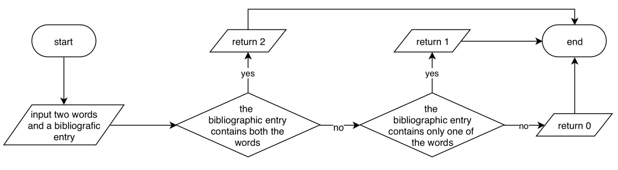
Fig. 20 The algorithm implemented with a flowchart.

Assess: check if the flowchart returns the correct output

After developing the flowchart, it is essential to test it by running it using the input defined in the step “Emulate”. We can act as a computer by executing the instructions in the flowchart. If the output values returned are the ones we expected, we can proceed to the next step (“Translate”). Otherwise, if some execution returned an unexpected output, we need to go back to the previous step and change something in the flowchart.

Executing the flowchart in Fig. 20 with the set of inputs mentioned in the example in step “Emulate”, all the output returned by each execution are compliant with the expected outcomes.

Translate: convert the flowchart into Python

In this step, we convert all the various instructions depicted by the flowchart widgets into particular Python constructs. In particular, the input widget should have been already converted into the parameters of the empty Python function developed in step “Fail”. The output widgets must be translated by using the return instruction. An if-else conditional block must express each decision widget. At the same time, the process widgets must be defined as simple Python instructions (e.g. assignments to variables). Listing 19 presents the full implementation of the algorithm in Python.

Succeed: check if the Python code returns the correct output

Finally, we should test the Python implementation of the algorithm according to the tests developed in step “Fail”. If all the output values returned by running the Python tests comply with the expected results, we have finished. Otherwise, if some execution returned an unexpected output, we need to go back to the previous step and change something in the Python implementation of the algorithm.

All the tests initially introduced in Listing 21 are passed as expected in the final code introduced in Listing 19. It is possible to use Python Tutor to see a complete execution of such code.

References

[Bec03]

Kent Beck. Test-driven development: by example. The Addison-Wesley signature series. Addison-Wesley, Boston, MA, USA, 2003. ISBN 978-0-321-14653-3. URL: https://archive.org/details/est-driven-development-by-example/test-driven-development-by-example/.

[MR11]

Bradley N. Miller and David L. Ranum. Problem solving with algorithms and data structures using Python. Franklin, Beedle & Associates, Wilsonville, OR, 2. ed edition, 2011. ISBN 978-1-59028-257-1. URL: https://runestone.academy/ns/books/published/pythonds/index.html.

[Pil09]

Mark Pilgrim. Dive into Python 3. The expert's voice in open source. Apress, New York, NY, USA, 2009. ISBN 978-1-4302-2415-0. URL: https://diveintopython3.net/.

[Tag18]

Lisa Tagliaferri. How to code in Python 3. DigitalOcean, New York, NY, USA, 2018. ISBN 978-0-9997730-1-7. OCLC: 1020289950. URL: https://assets.digitalocean.com/books/python/how-to-code-in-python.pdf.

Notes

---

[1]

The word boolean was named after George Boole, who was a great logician of the 19^th century.