Brute-force algorithms

This chapter introduces the notion of brute-force algorithms by implementing two algorithms of this kind: linear search and insertion sort. The historic hero introduced in these notes is Betty Holberton. She was one of the first programmers of the ENIAC and one of the key people for the development of several programming languages and algorithms for sorting objects.

Note

The slides for this chapter are available within the book content.

Historic hero: Betty Holberton

Frances Elizabeth – known as Betty – Holberton, shown in Fig. 24, was one of the first programmers of the Electronic Numerical Integrator and Computer (ENIAC). The funds of the United States Army permitted the development of this earliest electronic and general-purpose computer between 1943 and 1946. Besides, she contributed to developing several programming languages, such as COBOL and FORTRAN. In addition, she created the first statistical analysis tool used to analyse the United States Census data in 1950.

She dedicated a considerable part of her work to developing algorithms for sorting the elements in a list. The activity of sorting things is a typical human activity. It can be, of course, automatised using computers, and it is a desirable property to have for addressing several tasks.

Fig. 24 Picture of Betty Holberton in front of the ENIAC. Source: Wikimedia Commons.

Of course, sorting things is an expensive task, in particular, if you have to order billions of items. However, having such items sorted is crucial for several activities that we can perform on the list that contains them. For instance, in libraries, books are ordered according to specific guidelines such as the Dewey classification. Such a classification allows one to cluster books according to particular fields, and each cluster contains books ordered according to the authors’ names and the book title. With this kind of order, the librarian can find a requested title, avoiding looking at the billion books available one by one, thus saving a considerable amount of time, after all. Therefore, to sort things in advance is a good practice if one has to search these things several times in the future.

May the (brute) force be with you

In this chapter, for the very first time, we start to talk about problem-solving methods. In Computer Science, problem-solving is to create a computer-interpretable process (i.e. an algorithm) for solving some given problem, e.g. ordering all the books alphabetically in a library. Computer scientists have proposed several different methods for solving problems, grouped into general categories. Probably, the more uncomplicated class of problem-solving techniques is the brute-force approach.

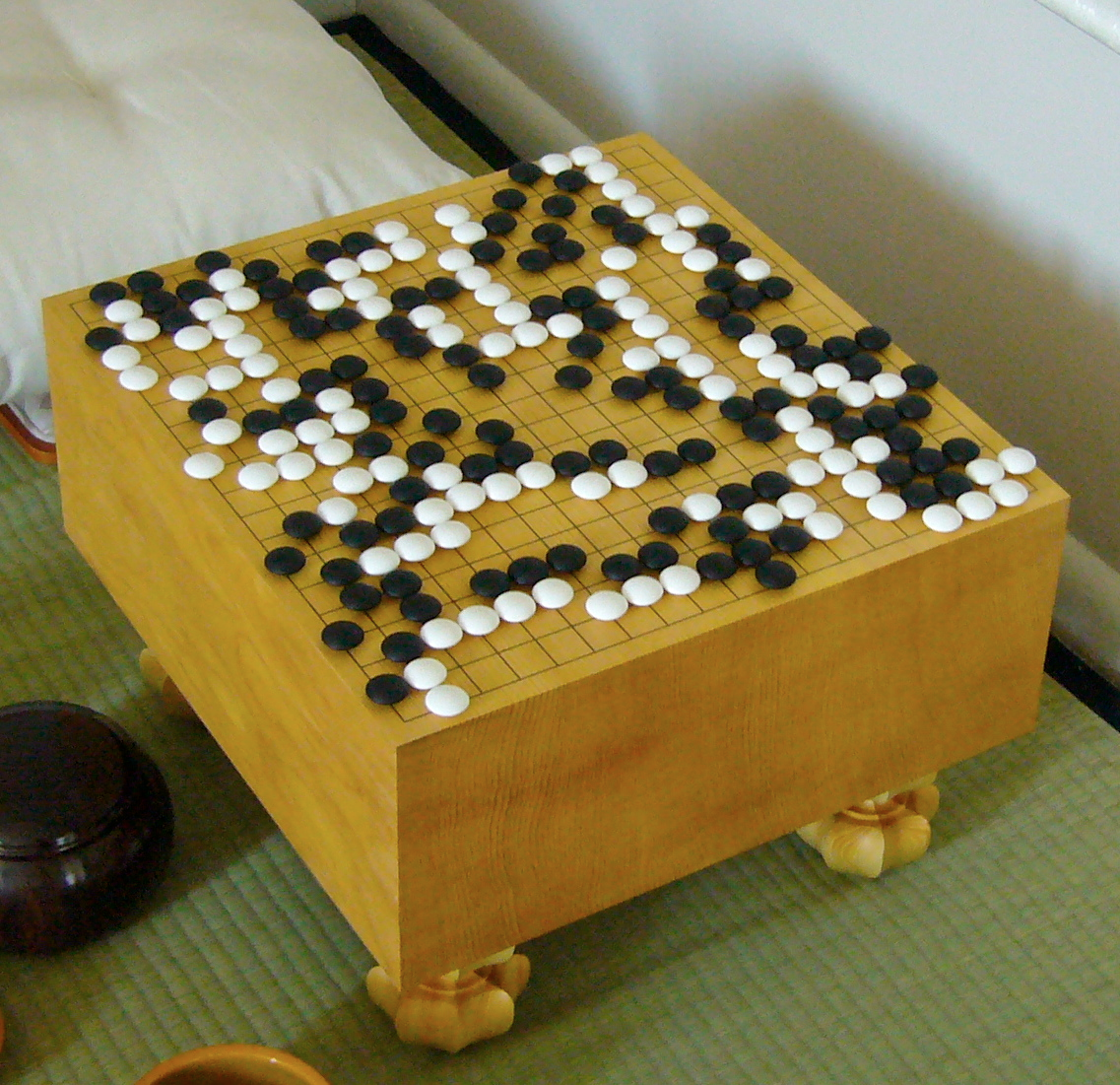
Fig. 25 The game of Go, which cannot be solved efficiently through a brute-force approach. Picture by Goban1, source: Wikimedia Commons.

Brute-force algorithms are these processes that reach the perfect solution to a problem by analysing all the possible candidate solutions. There are advantages and disadvantages to adopting such kind of approach. Usually, a brute-force approach is simple to implement, and it will always find a solution to the computational problem by considering iteratively all the possible solutions one by one. However, its computational cost depends strictly on the number of available candidate solutions. Thus, it is often a relatively slow, even if simple, approach for practical problems with a vast solution space. A good suggestion is to use such a brute force approach when the problem size is small.

Abstract strategy board games, such as Chess or Go, belong to that set of computational problems that have a pretty huge solution space. Writing a brute-force algorithm that can play the game appropriately requires considering all the possible legal moves available on the board (shown in Fig. 25). According to John Tromp, the number of all the possible legal moves in Go was determined to be \(10^{170}\) [Tro16]. That makes a brute-force approach intractable, even for an electronic computer.

Python has two alternatives for creating iterative blocks: for-each loops and while loops. The first kind of iteration mechanism is provided in Python through for statement, illustrated in Listing 24. All the instructions within the for block are repeated for each item in a collection (a list, a queue, etc.).

Listing 24 The general structure of a for-each loop in Python.

for item in <collection>:
    # do something using the current item`​

Listing 25 A simple function that takes a list as input and creates a stack with all the list’s values using a for-each loop. The source code of this listing is available as part of the material of the course.

from collections import deque

def stack_from_list(input_list):
    output_stack = deque()  # the stack to create


    # Iterate each element in the input list and add it to the stack
    for item in input_list:
        output_stack.append(item)

    return output_stack

The for-each loop is handy when we want to iterate on all the elements of a list. For instance, one can apply some operations on each or find a particular value – as discussed in more detail in Section linear-search. Or, we can use a for-each loop for creating a stack with all the elements included in a list, as shown by the simple algorithm in Listing 25.

Listing 26 The general structure of a while loop in Python.

while <condition>:
    # do something until the condition is true

The while loop, instead, works in a slightly different way. Python allows us to create it by using a while statement (as shown in Listing 26). The while statement will repeat all the instructions in such block until the condition specified is true. For instance, it is possible to use a while statement for implementing the run_forever function that maps the Turing machine introduced in Chapter Computability. Listing 27 shows one of its possible implementation in Python.

Listing 27 Another simple algorithm that sums 1 to a starting value indefinitely. The source code of this listing is available as part of the material of the course.

def run_forever():
    value = 0
    while value >= 0:
        value = value + 1

In the following sections, we reuse some of these iterations to implement two brute-force algorithms for searching the position of an item in a list and ordering a list. These are known as linear search and insertion sort.

Linear search

Searching for the position in which a particular value is in a list is an ordinary operation, which has applications in several real-life tasks. For instance, consider again the library’s example introduced in Section Historic hero: Betty Holberton. Once a librarian has received a particular request for a book, she consults the catalogue of all the library books. Then, she finds the appropriate location of the requested book. This scenario is a sort of actual application of the aforementioned abstract problem of searching a value in a list, which is formally defined as follows:

Computational problem

Find the position of the first occurrence of a value within a list.

While several approaches can be used to find an element in a list, we focus on a particular algorithm, called linear search. This approach is pretty simple. The idea is to iterate over all the items contained in an input list one by one. Then, one must check if they are equal to the value we are looking for, specified as input. Once the input value is found in the list, the librarian returns its position in the list. If the list does not contain the input value, she returns no position at all.

We need to clarify some aspects of the description of the linear search algorithm before providing its implementation in Python. The first one is that an item in a list has a specific position, which is quite natural if you think about it. However, in the previous chapter, we have not mentioned how to get such a position. Besides, there is an aspect typical of Computer Science: that wants to number every position starting from 0, instead of 1. Thus, for instance, looking at the books in Fig. 26, Terry Pratchett’s The Carpet People has position 0, James Ponti’s Dead City has position 1, and so on.

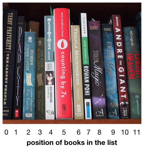
Fig. 26 The position numbers assigned to a book of a list according to the typical Computer Science habit – which starts numbering from 0.

Listing 28 How Python allows one to decouple tuples in for-each loops involving a collection of tuples by assigning a variable to each item in the tuple.

for <var_item_1>, <var_item_2>, ... in <collection of tuples>:
    # here you can use directly the variables defining 
    # the various items in the tuple​

Python allows one to use the function enumerate(<list>) for retrieving an item’s current position in a list that is accessed using a for-each loop. This function takes a list of values as input and returns a kind of list (it is an enumerate object: it behaves like a list, but it is not a list) of tuples. Each tuple contains two elements: the first element is the position of the item in consideration within the list, while the second element is the item itself. In Python, a tuple is created by specifying comma-separated values between round brackets – for instance, my_tuple = (0, 1, 2, 3, 4, 5) assigns a tuple with six numbers to my_tuple. Thus, while tuples could be perceived as similar to lists, they are not. The main difference with lists is that tuples do not provide any way for updating them with a new value since they do not permit the append operation. Thus, once a tuple is created, it stays forever.

Listing 29 The linear search algorithm described in Python, including its test case. The source code of this listing is available as part of the material of the course.

# Test case for the algorithm
def test_linear_search(input_list, value_to_search, expected):
    result = linear_search(input_list, value_to_search)
    if expected == result:
        return True
    else:
        return False

# Code of the algorithm
def linear_search(input_list, value_to_search):
    # iterate all the items in the input list, 
    # getting also their position on the list
    for position, item in enumerate(input_list):
        # check if the current item is equal to the value to search
        if item == value_to_search:
            # if so, the position of the current item is returned 
            # and the algorithm stops
            return position

# Three different test runs
print(test_linear_search([1, 2, 3, 4, 5], 3, 2))
print(test_linear_search(["Alice", "Catherine", "Bob", "Charles"], 
                          "Denver", None))
print(test_linear_search(["Ron", "Harry", "Hermione"], "Ron", 0))

Considering these aspects, running the function enumerate(list(["a", "b", "c"])) will return the following enumeration of tuples: enumerate([(0, "a"), (1, "b"), (2, "c")]), where the first item of each tuple is the position that the second item of the tuple has in the original list. Also, Python allows us to decouple the items in a tuple by specifying names for each item with variables created in the for statement on the fly, as shown in Listing 28. Thus, for instance, a for-each loop like for position, item in enumerate([(0, "a"), (1, "b"), (2, "c")]) will assign 0 to ​position and “a” to ​item in the first iteration, 1 to ​position and “b” to ​item in the second iteration, and 2 to ​position and “c” to ​item in the third iteration.

Listing 30 An example of the execution steps of the linear search algorithm implemented.

​list_of_books = list(["Coraline", "American Gods", 
                      "The Graveyard Book", "Good Omens", 
                      "Neverwhere"])

​​linear_search(list_of_books, "The Graveyard Book")
​
​# FOR-EACH LOOP EXECUTION
​# enumerate(input_list) will result in: 
​# enumerate([(0, "Coraline"), (1, "American Gods"), 
#            (2, "The Graveyard Book"), (3, "Good Omens"), 
#            (4, "Neverwhere")])
​#
​# Iteration 1
​# position = 0
​# item = "Coraline"
​# item == value_to_search is False
​# Continue to the next iteration
​#
​# Iteration 2
​# position = 1
​# item = "American Gods"
​# item == value_to_search is False
​# ​Continue to the next iteration
​#
​# Iteration 3
​# position = 2
​# item = "The Graveyard Book"
​# item == value_to_search is True
​# Return the position (i.e. 2) and end the execution of the algorithm

There is an aspect that is implicit in the description of the linear search algorithm introduced before. Indeed, the algorithm should not return any position if the value to search is not present in the list. In Python, this can be implemented by returning nothing (i.e. by not ever executing the statement return) or explicitly returning a particular object that means nothing, i.e. None.

At this point, we have all the ingredients for developing the linear search algorithm in Python, shown in Listing 29. To understand how the algorithm works, we have prepared a description of the various execution steps (shown in Listing 30) of the for-each loop introduced in the algorithm. This description would allow the reader to glance at how iterative loops work from a purely computational point of view.

Insertion sort

As already mentioned in Section Historic hero: Betty Holberton, the task of ordering a sequence of items is an operation we usually have to deal with in everyday life. Recalling the library’s example, having the books sorted will make searching them more efficient. It would allow us to avoid using naive approaches for the search, e.g. the one introduced in Section linear-search. These naive approaches are pretty expensive if we have billions of books to check.

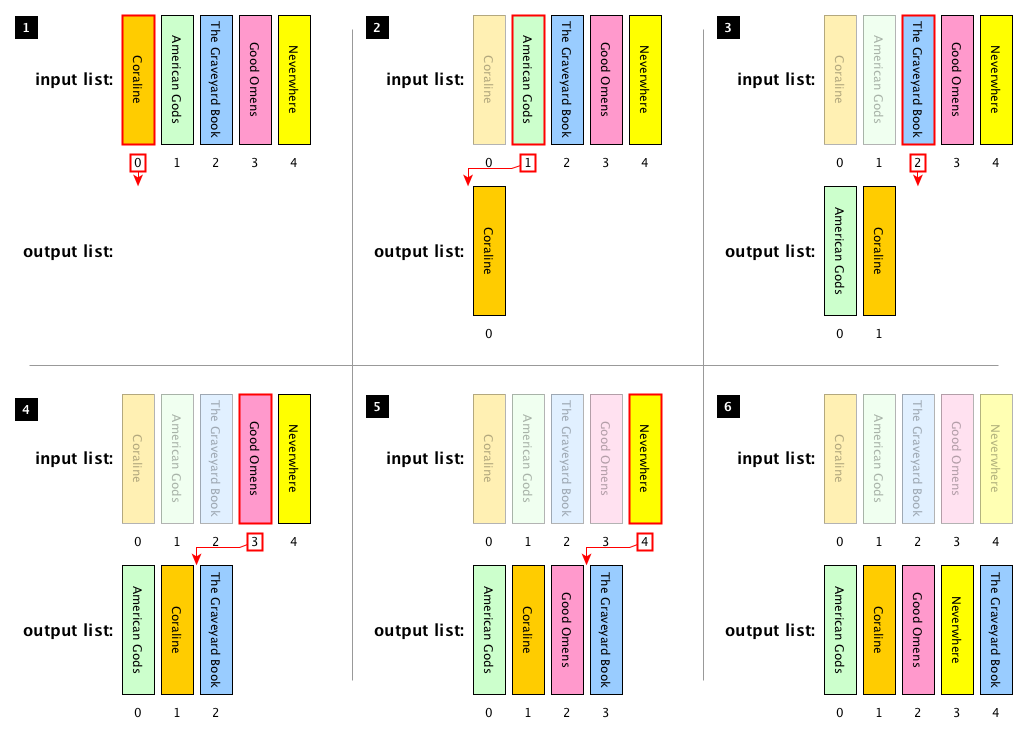
Fig. 27 The execution of the insertion sort algorithm using the following list of book titles as input: Coraline, American Gods, The Graveyard Book, Good Omens, Neverwhere. The book highlighted by a bold red border is currently selected in the particular iteration of the algorithm. The red arrow shows the assigned position of the book in the output list. We use a transparent filter on books considered in previous iterations of the process.

In this section, we propose one particular brute-force algorithm for addressing the following computational problem:

Computational problem

Sort all the items in a given list.

The algorithm that we want to use for addressing the aforementioned computational problem is called insertion sort. It is one of the simplest sorting algorithms to implement[1], and it is pretty efficient for small lists. The idea behind this algorithm is the following. First, it considers the items in the list one by one, according to the order placed. Thus, at each iteration, it removes one item from the input list. Then, it finds the correct location in the output list by looking at the items the output list contains starting from the last one (i.e. the rightmost one). Finally, it inserts it in the location found. The algorithm finishes when there are no more items to add to the output list. Fig. 27 shows an example of the execution of this algorithm.

Listing 31 The insertion sort algorithm described in Python. The source code of this listing is available as part of the material of the course and includes the algorithm’s test case.

def insertion_sort(input_list):
    result = list()  # A new empty list where to store the result

    # iterate all the items on the input list
    for item in input_list:

        # initialise the position where to insert the item 
        # at the end of the result list
        insert_position = len(result)

        # iterate, in reverse order, all the positions of all the
        # items already included in the result list
        for prev_position in reversed(range(insert_position)):

            # check if the current item is less than the one in 
            # prev_position in the result list
            if item < result[prev_position]:
                # if it is so, then the position where to insert the 
                # current item becomes prev_position
                insert_position = prev_position

        # the item is inserted into the position found
        result.insert(insert_position, item)

    return result  # the ordered list is returned

To provide a Python implementation of this algorithm, we need to introduce two functions and one additional operation applicable to lists. The first function we need to use is range(<stop_number>). It takes a non-negative number as input. It returns a kind of list (i.e. a range object behaving like a list) of all numbers from 0 to the one preceding stop_number. Thus, for instance, range(4) returns the range([0, 1, 2, 3]), while range(0) returns the empty range object range([]).

The other function is reversed(<input_list>). This function takes a list as input. It returns a kind of list, i.e. an iterator for iterating the items in the list in reversed order. Thus, for instance, reversed(list([0, 1, 2, 3])) returns iterator([3, 2, 1, 0]). We can use these two functions in combination. They allow us to obtain the positions of the items already ordered in past iterations of the algorithm. For instance, reversed(range(2)) returns iterator(range([1, 0])) starting from the position (i.e. 2) of the third item in the input list.

In addition, we need a way for selecting an item in a list and for inserting an item in a specific position in a list. For addressing these tasks, Python makes available the additional list methods <list>[<position>] and <list>.insert(<position>, <item>). In particular, the former returns the item in the list at the specified position – e.g. if we have the list ​my_list = list(["a", "b", "c"]), ​my_list[1] returns “b”. The latter method allows one to put <item> in the position specified, and it shifts all the elements with position greater than or equal to <position> of one position – e.g., by applying my_list.insert(1, "d"), the list in my_list is modified as follows: list(["a", "d", "b", "c"]).

At this point, we have all the ingredients for developing the insertion sort algorithm in Python, shown in Listing 31.

References

[Tro16]

John Tromp. Counting Legal Positions in Go. 2016. URL: http://tromp.github.io/go/legal.html.

Notes

---

[1]

For a more comprehensive discussion and examples on sorting algorithms, please see the Visualgo webpage about them and a creative Youtube video showing fifteen distinct sorting algorithms in action.