Divide and conquer algorithms#
This chapter introduces the notion of divide and conquer algorithms by implementing one algorithm of this kind: merge sort. The historic hero introduced in these notes is John von Neumann. He proposed a set of guidelines for the designing of the EDVAC named after him. These guidelines have been fundamental design principles for building the first electronic computers.
Note
The slides for this chapter are available within the book content.
Historic hero: John von Neumann#
John von Neumann (depicted in Fig. 36) was a computer scientist, mathematician, and physicist. He was very active in all these disciplines. In addition, he made an incredibly huge number of contributions in several fields, such as quantum mechanics, game theory, and self-replicating machines.
One of his most important and famous contributions in the Computer Science domain was the digital computer architecture named after him [vN45]. He wrote about it for the very first time in an incomplete document for defining the main design principles of the Electronic Discrete Variable Automatic Computer (EDVAC), the binary-based successor of the ENIAC. Von Neumann’s architecture has been used as the main guidelines for building several electronic computers in the following years and still represent an excellent approximate model for describing several of the main components of today’s digital computers.
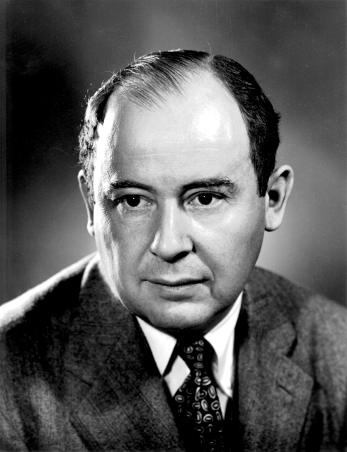
Fig. 36 A picture of John von Neumann at Los Alamos. Source: Wikimedia Commons.#
He also made other crucial contributions in Computer Science, such as the merge sort algorithm we introduce in this chapter. Also, he was one of the people involved in the top-secret Trinity project and its related parent project, i.e. the Manhattan Project, during World War II.
Clarification: immutable and mutable values#
We have introduced the mutability and immutability of Python objects when talking about lists and tuples. A mutable object (e.g. a list) is an object that can change in time – we can create an empty list, populate it with new values, remove some of them, etc. On the other hand, an immutable object, like a tuple, is that entity that, once it is created, cannot be further modified. In particular, we can group Python basic types in the following way:
strings, numbers, booleans, None, and tuples are immutable;
lists, sets, and dictionaries are mutable.
as part of the material of the course.# 1def add_one(n):
2 n = n + 1
3 return n
4
5my_num = 41
6print(my_num) # 41
7
8result = add_one(my_num)
9print(my_num) # 41
10print(result) # 42
as part of the material of the course.# 1def append_one(lst):
2 lst.append(1)
3 return lst
4
5my_list = list()
6my_list.append(2)
7print(my_list) # list([2])
8
9result = append_one(my_list)
10print(my_list) # list([2, 1])
11print(result) # list([2, 1])
This distinction is crucial when we use these kinds of objects as an input of functions or methods. They are handled in different ways, depending on dealing with mutable or immutable types. For instance, in the snippet of code in Listing 43, a simple function sums 1 to the number passed as input and then returns it. However, we always use the same variable n to store the operation’s result before returning it. Since numbers are immutable, the actual value associated with the original my_num, used as the input of the function def add_one(n), is not modified due to the function’s execution. This behaviour is the way (i.e. by value) Python uses to handle immutable values when passed as input of functions. It means that Python copies the value associated with the variable my_num to the variable that defines the function’s input parameter, i.e. n, before executing the code of the function itself.
Contrarily, mutable objects work in a slightly different way. For example, in the snippet of code in Listing 44, Python does not copy the list specified in the variable my_list (a mutable object), used as the input of the function def append_one(lst), into the variable defining the input parameter of the function, i.e. lst. Instead, Python references to it by such input parameter – i.e. both my_list and lst refer to the same list. This behaviour is the way (i.e. by reference) Python uses to handle mutable values when passed as input of functions.
We have a similar behaviour when assigning immutable and mutable values to a particular variable, as shown in Listing 45. One can observe how these executions and assignments affect the related objects by running all the codes in this section using Python Tutor.
as part of the material of the course.# 1# Immutable objects
2my_num_1 = 41
3my_num_2 = my_num_1
4my_num_1 = my_num_1 + 1
5print(my_num_1) # 42
6print(my_num_2) # 41, since it is a copy of the original value
7
8# Mutable objects
9my_list_1 = list()
10my_list_2 = my_list_1
11my_list_1.append(1)
12print(my_list_1) # [1]
13print(my_list_2) # [1], since it points to the same list
Ordering billions of books#
In one of the previous chapters, we have introduced an algorithm for ordering the items in a list called insertion sort. It is pretty simple – even natural, we could say. This algorithm works exceptionally well when the size of the list is small, but it is not very efficient when we have to deal with an incredibly significant amount of data. This behaviour is due to the brute-force approach it is implementing. While relatively simple, the mechanism followed by the insertion sort obliges a computer to scan the list several times for constructing an ordered list from an unordered one.
However, the insertion sort is not the only algorithm proposed for ordering the items in a list. Other relatively efficient approaches have been developed in the past to perform a better (and quicker) sorting of list items in a more reasonable time – even for an electronic computer. Some of these algorithms works if particular pre-conditions hold – such as specifying the number of buckets for the bucket sort algorithm.
Divide and conquer sorting algorithms are among those that behave efficiently well on large input lists. Divide and conquer is an algorithmic technique. It splits the original computational problem to solve in two or more smaller problems of the same type until they become solvable directly by executing a simple set of operations. Potentially, such smaller problems can be addressed in parallel by different computers (e.g. humans). Then, the solutions to these sub-problems are recombined to provide the answer to the original problem. Any divide and conquer algorithm is based on the recursive call of the very same algorithm, according to the following (informal) steps:
[base case] address the problem directly on the input material if it is depicting an easy-to-solve problem; otherwise
[divide] split the input material into two or more balanced parts, each representing a sub-problem of the original one;
[conquer] run the same algorithm recursively for every balanced part obtained in the previous step;
[combine] reconstruct the final solution of the problem using the partial solutions obtained from running the algorithms on the smaller parts of the input material.
There are several divide and conquer sorting algorithms. In this chapter, we introduce just one of these: the merge sort.
Merge sort#
John von Neumann proposed the merge sort (or mergesort) algorithm in 1945. It implements a divide a conquer approach for addressing the following computational problem (that we have already seen when we have introduced the insertion sort):
Computational problem
Sort all the items in a given list.
Unlike the insertion sort, the sorting approach defined by the merge sort is less intuitive. Still, it is more efficient, even considering an extensive list as input. In particular, the merge sort is a recursion-based algorithm – like any other divide and conquer approach – and uses another ancillary algorithm in its body, called merge. This latter algorithm is responsible for combining two ordered input lists to return a new list that contains all the elements in the input lists ordered. The following steps illustrate the loop suggested by this algorithm to create such a new list:
consider the first items of both the input lists;
remove the lesser item from the related list and append it into the result list
if the input list from where we removed the item is not empty, repeat from 1, otherwise append all the items of the other input list to the result list.
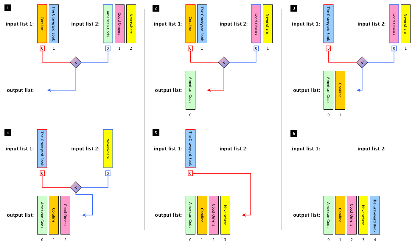
Fig. 37 The process of merging two ordered lists of books together in a new list having all books ordered.#
In Fig. 37, we illustrate the execution of the algorithm merge graphically by using two lists of books as inputs, i.e. list(["Coraline", "The Graveyard Book"]) and list(["American Gods", "Good Omens", "Neverwhere"]) respectively. In particular, the first four steps of the execution start creating the output list by comparing the first items of the input lists at each iteration of the loop. Then, in the 5th step, all the items of the only non-empty input list are appended to the output list in the order they appear in the input list. Finally (step 6), the output list is completed and is returned. Listing 46 shows the implementation in Python of the merge algorithm.
The merge algorithm is used in the merge sort to reconstruct a solution from two partial ones. In particular, the steps composing the algorithm[1] can be summarised as follows:
[base case] if the input list has only one item, return the list as it is; otherwise,
[divide] split the input list into two balanced halves, i.e. containing almost the same number of items each;
[conquer] run the merge sort algorithm recursively on each of the halves obtained in the previous step;
[combine] merge the two ordered lists returned by the last step by using the algorithm merge and return the result.
as part of the material of the course and includes the related test cases.# 1def merge(left_list, right_list):
2 result = list()
3
4 # Repeat until both lists have at least one item
5 while len(left_list) > 0 and len(right_list) > 0:
6 left_item = left_list[0]
7 right_item = right_list[0]
8
9 # If the item in left_list is less than the one in right_list,
10 # add the formed to the result and remove it from left_list
11 if left_item < right_item:
12 result.append(left_item)
13 left_list.remove(left_item)
14 # Otherwise, the item in right_list is added to the result and
15 # removed from the right_list
16 else:
17 result.append(right_item)
18 right_list.remove(right_item)
19
20 # Add to the result the remaining items from the lists
21 result.extend(left_list)
22 result.extend(right_list)
23
24 return result
In Fig. 38, we illustrate the execution of the merge sort algorithm graphically by using one list of books as inputs, i.e. my_list = list(["The Graveyard Book", "Coraline", "Good Omens", "Neverwhere", "American Gods"]). Before introducing the implementation in Python of the algorithm, we must clarify some operations that we will use to create the balanced halves from the input list.
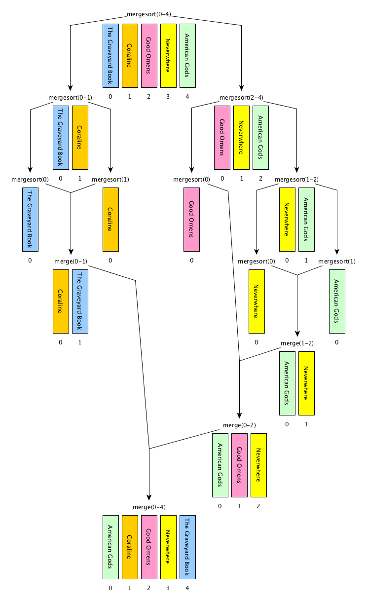
Fig. 38 A graphical execution of the merge sort algorithm, which reuses the merge algorithm implemented by the function def merge(left_list, right_list) introduced in Listing 46.#
as part of the material of the course and also includes the related test cases.# 1# Import the function 'merge'
2# from the module 'merge' (file 'merge.py')
3from merge import merge
4
5# Code of the algorithm
6def merge_sort(input_list):
7 input_list_len = len(input_list)
8
9 # base case: the list is returned if it is empty or
10 # contain just one element
11 if len(input_list) <= 1:
12 return input_list
13 # recursive case
14 else:
15 # the floor division of the length, returning the quotient
16 # in which the digits after the decimal point are removed
17 # (e.g. 7 // 2 = 3)
18 mid = input_list_len // 2
19
20 # iterative steps, running the merge_sort on the
21 # sublists split by mid
22 left = merge_sort(input_list[0:mid])
23 right = merge_sort(input_list[mid:input_list_len])
24
25 # merge the two (ordered) lists and return the result
26 return merge(left, right)
The first operation is the floor division between two numbers, i.e. <number_1> // </number_2>. It works like any common division, except that it returns only the integer part of the result number discarding the fractional part. For instance, 3 // 2 will be 1 (i.e. 1.5 without its fractional part), 6 // 2 will be 3 (since its fractional part is 0), and 1 // 4 will be 0 (i.e. 0.25 without its fractional part).
The second operation allows us to create on-the-fly a new list from a selection of the elements in an input list: <list>[<start_position>:<end_position>]. Basically speaking, this operation creates a new list containing all the elements in <list> that range from <start_position> to <end_position> - 1. For instance, considering the aforementioned list in my_list, my_list[0:2] returns list(["Coraline", "The Graveyard Book"]) while my_list[2:5] returns list(["American Gods", "Good Omens", "Neverwhere"]). It is worth mentioning that the <list> won’t be modified by such an operation.
Thus, now we have all the ingredients for introducing the Python implementation of the merge sort algorithm. Listing 47 illustrates the function def merge_sort(input_list).
References#
Sándor P. Fekete and blinry. MERGE SÖRT. January 2018. URL: https://idea-instructions.com/merge-sort/.
John von Neumann. First Draft of a Report on the EDVAC. Technical Report, University of Pennsylvania, Philadelphia, PA, USA, June 1945. URL: https://web.archive.org/web/20130314123032/http://qss.stanford.edu/~godfrey/vonNeumann/vnedvac.pdf (visited on 2025-10-11).