Part 4: Exercises

Exercise 50

The variable my_list contains a list of ten integer number from 0 to 9. Study the execution of the following function when it is called as algorithm(my_list, 0):

def algorithm(a_list, pos):
    if pos >= len(a_list):
        return a_list
    else:
        common_division = pos / 2
        floor_division = pos // 2
        if floor_division < common_division:
            a_list.remove(a_list[floor_division])

        return algorithm(a_list, pos + 1)

Solution to Exercise 50

The recursive function algorithm modifies the list in input according to the particular position in the list specified, until all the items in the list have been processed. The first call starts working on the very first item of the list, thus starting with the instructions in the else block - unless the initial list is empty (in this case, the empty list will be returned as such).

The instructions in the else check if the position (i.e. pos) is an odd number and, in that case, it modify the list removing the first instance of the item in position pos // 2. Independently from the fact that the execution remove an item or not from the input list, the last step execute a recursive step calling the function algorithm passing the list (modified or not) and a subsequent position (i.e. pos + 1) as input, and returns the value returned by the recursive execution.

For instance, the following call

my_list = [0, 0, 0, 1, 0, 9, 8, 2, 0, 7]
result = algorithm(my_list, 0)
print(result)

prints on screen the list [1, 0, 9, 8, 2, 0, 7].

The source Python file of the code shown above is available as part of the material of the course. You can run it executing the command python ex-und-modify_list.py in a shell.

Exercise 51

The variable my_mat_string contains a string of ten 0-9 digits (e.g. "0000123456"). Study the execution of the following functions when they are called as follows: f(my_mat_string).

def f(mat_string):
    c = 0
    lst = list()

    for chr in mat_string:
        n = int(chr)
        lst.append(n)
        if n / 2 != n // 2:
            c = c + 1

    return g(lst, c)


def g(mat_list, c):
    if c <= 0 or len(mat_list) == 0:
        return 0
    else:
        v = 0
        result = list()

        for i in mat_list:
            if v > 0:
                result.append(i)
            if i > 0 and v == 0:
                v = i

        return v + g(result, c - 1)

Solution to Exercise 51

The function f transform the input string in another data structure, i.e. a list of integers (created casting the digit character into the related number) and counts the number of odd numbers the list contains (using the variable c). The function g, that is called by the function f, is a recursive function.

The instructions that are executed by the function g, in case the input list is not empty and the input number is greater than 0, creates a new list. In particular, it iterates over all the numbers of the input list. At every iteration, the current number considered (i.e. i) is added to the new list if the variable v, set to 0 before starting the for each loop, is greater than 0. In addition, the variable v is updated with the value of the variable i during the first iteration in which i assumes a value greater than 0. Thus, the for each loop create a sublist of the original input list that includes all the elements in the input list starting from the item following the one considered when v is modified.

Finally, the recursive step is executed, passing the new list created and c - 1 as input, and the result is summed to the value specified in the variable v and then returned.

For instance, the following call

my_mat_string = "0001098207"
result = f(my_mat_string)
print(result)

prints on screen the number 18.

The source Python file of the code shown above is available as part of the material of the course. You can run it executing the command python ex-und-number_from_matriculation.py in a shell.

Exercise 52

The Euclidean algorithm is a method for computing the greatest common divisor (GCD) of two integers, i.e. the largest number that divides them both without a remainder.

The Euclidean algorithm is based on the principle that the GCD of two numbers does not change if the larger number is replaced by its difference with the smaller number. For example, 3 is the GCD of 15 and 6 (as 15 = 3 × 5 and 6 = 3 × 2), and the same number 3 is also the GCD of 6 and 15 − 6 = 9. Since this replacement reduces the larger of the two numbers, repeating this process gives smaller pairs of numbers successively until the two numbers become equal. When that occurs, that number is the GCD of the original two numbers:

1. GCD(15, 6) = GCD(15-6=9, 6)

2. GCD(9, 6) = GCD(9-6=3, 6)

3. GCD(3, 6) = GCD(3, 6-3)

4. GCD(3, 3) = 3

Write a recursive algorithm in Python – def euclidean(r, s) – which takes in input two integer numbers s and r greater than zero, and returns their greatest common divisor. Accompany the implementation of the function with the appropriate test cases.

Solution to Exercise 52

# Test case for the function
def test_euclidean(r, s, expected):
    result = euclidean(r, s)
    
    if result == expected:
        return True
    else:
        return False


# Code of the function
def euclidean(r, s):
    if r == s:
        return r
    elif r < s:
        return euclidean(r, s - r)
    else:
        return euclidean(r - s, s)

        
# Tests
print(test_euclidean(1, 1, 1))
print(test_euclidean(1, 2, 1))
print(test_euclidean(1, 3, 1))
print(test_euclidean(3, 2, 1))
print(test_euclidean(3, 3, 3))
print(test_euclidean(3, 9, 3))
print(test_euclidean(15, 6, 3))

The source Python file of the code shown above is available as part of the material of the course. You can run it executing the command python ex-dev-euclidean.py in a shell.

Exercise 53

Write down, using a divide and conquer approach, the body of the following Python function:

def sum(number_list) 

The function takes a list of numbers as input and returns their sum. The use of any form of iteration (e.g. for each and while loops) is prohibited. Accompany the implementation of the function with the appropriate test cases.

Solution to Exercise 53

# Test case for the function
def test_sum(number_list, expected):
    result = sum(number_list)
    if expected == result:
        return True
    else:
        return False


# Code of the function
def sum(number_list):
    list_len = len(number_list)
    
    if list_len == 0:
        return 0
    elif list_len == 1:
        return number_list[0]
    else:
        mid = list_len // 2
        return sum(number_list[0:mid]) + sum(number_list[mid:list_len])


# Tests
print(test_sum([9, 9, 9], 27))
print(test_sum([8, 5, 9, 8, 3, 6], 39))
print(test_sum([], 0))
print(test_sum([42], 42))

The source Python file of the code shown above is available as part of the material of the course. You can run it executing the command python ex-dev-sum.py in a shell.

Exercise 54

Implement in Python the binary search algorithm – i.e. the recursive function def binary_search(item, ordered_list, start, end).

It takes an item to search (i.e. item), an ordered list and starting and ending positions in the list as input. It returns the position of item in the list, if it is in the list, and None otherwise. The binary search first checks whether the middle item of the list between start and end (inclusive) is equal to item, and returns its position if so. Otherwise, if the middle item is less than item, the algorithm continues the search in the part of the list that follows the middle item. Instead, in case the middle item is greater than item, the algorithm continues the search in the part of the list that precedes the middle item. Accompany the implementation of the function with the appropriate test cases.

As supporting material, Fekete and blinry released a nonverbal definition of the algorithm [Fblinry18a], which is useful to understand the rationale of the binary search steps.

Solution to Exercise 54

# Test case for the function
def test_binary_search(item, ordered_list, start, end, expected):
    result = binary_search(item, ordered_list, start, end)
    if expected == result:
        return True
    else:
        return False


def binary_search(item, ordered_list, start, end):
    if len(ordered_list) > 0 and start <= end:
        mid = (start + end) // 2
        mid_item = ordered_list[mid]
        if item == mid_item:
            return mid
        elif mid_item < item:
            return binary_search(item, ordered_list, mid + 1, end)
        else:
            return binary_search(item, ordered_list, start, mid - 1)


# Tests
print(test_binary_search(3, [1, 2, 3, 4, 5], 0, 4, 2))
print(test_binary_search("Denver", ["Alice", "Bob", "Catherine", "Charles"], 0, 3, None))
print(test_binary_search("Harry", ["Harry", "Hermione", "Ron"], 0, 2, 0))
print(test_binary_search("Harry", [], 0, 0, None))

The source Python file of the code shown above is available as part of the material of the course. You can run it executing the command python ex-binary_search.py in a shell.

Exercise 55

Implement in Python the partition algorithm – i.e. the non-recursive function def partition(input_list, start, end, pivot_position).

It takes a list and the positions of the first and last elements in the list to consider as inputs. It redistributes all the elements of a list having position included between ​start and ​end on the right of the pivot value input_list[pivot_position] if they are greater than it, and on its left otherwise. Also, the algorithm returns the new position where the pivot value is now stored. For instance, considering ​​my_list = list(["The Graveyard Book", "Coraline", "Neverwhere", "Good Omens", "American Gods"]), the execution of partition(my_list, 1, 4, 1) changes ​my_list as follows: ​list(["The Graveyard Book", "American Gods", "Coraline", "Neverwhere", "Good Omens"]) and 2 will be returned (i.e. the new position of "Coraline"). Note that "The Graveyard Book" has not changed its position in the previous execution since it was not included between the specified start and end positions (i.e. 1 and 4 respectively). Accompany the implementation of the function with the appropriate test cases.

As supporting material, Ang recorded a video which is useful to understand the rationale of the partition steps.

Solution to Exercise 55

# Test case for the function
def test_partition(input_list, start, end, pivot_position, expected):
    p_value = input_list[pivot_position]
    result = partition(input_list, start, end, pivot_position)
    output = expected == result and p_value == input_list[result]

    for item in input_list[0:result]:
        output = output and item <= p_value
    for item in input_list[result + 1:len(input_list)]:
        output = output and item >= p_value

    return output


# Code of the function
def partition(input_list, start, end, pivot_position):
    pivot_value = input_list[pivot_position]

    swap_index = start - 1
    for index in range(start, end + 1):
        if input_list[index] < pivot_value:
            swap_index += 1
            if swap_index == pivot_position:
                pivot_position = index
            swap(input_list, swap_index, index)

    new_pivot_position = swap_index + 1
    swap(input_list, pivot_position, new_pivot_position)

    return new_pivot_position


def swap(input_list, old_index, new_index):
    cur_value = input_list[old_index]
    input_list[old_index] = input_list[new_index]
    input_list[new_index] = cur_value


# Run tests
print(test_partition([1, 2, 3, 4, 5], 0, 4, 0, 0))
print(test_partition([4, 5, 3, 1, 7], 0, 4, 0, 2))
print(test_partition([4, 5, 3, 1, 7], 0, 4, 2, 1))
print(test_partition([7, 5, 3, 1, 4], 0, 4, 4, 2))
print(test_partition([1, 9, 7, 5, 9, 3, 1, 4, 2, 3], 0, 9, 1, 8))
print(test_partition([1, 9, 7, 5, 9, 3, 1, 4, 2, 3], 0, 9, 0, 0))
print(test_partition([1, 9, 7, 5, 9, 3, 1, 4, 2, 3], 0, 9, 3, 6))
print(test_partition([1, 2, 2, 3, 9, 8, 4], 1, 2, 1, 1))

The source Python file of the code shown above is available as part of the material of the course. You can run it executing the command python ex-partition.py in a shell.

Exercise 56

Implement in Python the divide and conquer quicksort algorithm – i.e. the recursive def quicksort(input_list, start, end)​.

It takes a list and the positions of its first and last elements as inputs. Then, it calls partition(input_list, start, end, start) (defined in the previous exercise) to partition the input list into two slices. Finally, it executes itself recursively on the two partitions (neither of which includes the pivot value since it has already been correctly positioned through the execution of partition). In addition, define the base case of the algorithm appropriately to stop if needed before running the partition algorithm. Accompany the implementation of the function with the appropriate test cases.

As supporting material, Fekete and blinry released a nonverbal definition of the algorithm [Fblinry18b], which is useful to understand the rationale of the quicksort.

Solution to Exercise 56

# Test case for the function
def test_quicksort(input_list, start, end, expected):
    result = quicksort(input_list, start, end)
    if expected == result:
        return True
    else:
        return False


# Code of the function
def quicksort(input_list, start, end):
    if start < end:
        pivot_position = partition(input_list, start, end, start)
        quicksort(input_list, start, pivot_position - 1)
        quicksort(input_list, pivot_position + 1, end)
    return input_list

def partition(input_list, start, end, pivot_position):
    pivot_value = input_list[pivot_position]

    swap_index = start - 1
    for index in range(start, end + 1):
        if input_list[index] < pivot_value:
            swap_index += 1
            if swap_index == pivot_position:
                pivot_position = index
            swap(input_list, swap_index, index)

    new_pivot_position = swap_index + 1
    swap(input_list, pivot_position, new_pivot_position)

    return new_pivot_position

def swap(input_list, old_index, new_index):
    cur_value = input_list[old_index]
    input_list[old_index] = input_list[new_index]
    input_list[new_index] = cur_value
    

# Run tests
print(test_quicksort([1], 0, 0, [1]))
print(test_quicksort([1, 2, 3, 4, 5, 6, 7], 0, 6, [1, 2, 3, 4, 5, 6, 7]))
print(test_quicksort([3, 4, 1, 2, 9, 8, 2], 0, 6, [1, 2, 2, 3, 4, 8, 9]))
print(test_quicksort(["Coraline", "American Gods", "The Graveyard Book", "Good Omens", "Neverwhere"], 0, 4,
                     ["American Gods", "Coraline", "Good Omens", "Neverwhere", "The Graveyard Book"]))

The source Python file of the code shown above is available as part of the material of the course. You can run it executing the command python ex-quicksort.py in a shell.

Exercise 57

Consider the following function:

def rin(g_name, f_name, idx):
    result = []

    if len(g_name) > 0:
        if g_name[0] in f_name:
            result.append(idx)
        
        idx = idx + 1
        result.extend(rin(g_name[1:len(g_name)], f_name, idx))

    return result 

The variable my_g_name contains the string with your given name in lower case (e.g. "john"), and my_f_name contains the string with your family name in lower case (e.g. "doe"). What is the value returned by calling the function sc as shown as follows:

rin(my_g_name, my_f_name, 0)

Solution to Exercise 57

The function rin is an recursive recursive function that reduces the characters of the given name at each recursive call, removing the first one. In particular, in each call (in case the g_name input parameter is not empty) it adds the value of idx to the result list in case the first character of g_name is also included in f_name. The final list returned will be a list of non-negative integers.

For instance, executing the function as follows

rin("john", "doe", 0)

returns the list [1].

The source Python file of the code shown above is available as part of the material of the course. You can run it executing the command python ex-und-given_and_family_names.py in a shell.

Exercise 58

Consider the following function:

def rsel(full_name, mat_string):
    uniq = []
    for c in full_name:
        if c not in uniq:
            uniq.append(c)
    
    r = []
    i = len(mat_string) // 2
    if i > 0:
        n = int(mat_string[i])
        if n < len(uniq):
            r.append(uniq[n])
            new_full_name = full_name[0:n] + full_name[n+1:len(full_name)]
            new_mat_string = mat_string[0:n] + mat_string[n+1:len(mat_string)]
            r.extend(rsel(new_full_name, new_mat_string))
    
    return r

The variable my_mat_string contains the string of all ten numbers of a matriculation number (e.g. "0235145398"), and my_full_name is a string of a full name, all in lowercase with no spaces (e.g. "johndoe"). Write down the value returned by calling the function rsel as shown as follows:

rsel(my_full_name, my_mat_string)

Solution to Exercise 58

The function rsel is a recursive function that, at every call, reduce both the input parameters of one character. In particular, it identifies all the unique letters in the given input string full_name, it sees if the mat_string contains at least two characters, and then it appends, to the list to be returned as result, the character in the list of unique letters that is specified in the position specified by the first digit number after the first half of the matricutation string if such position is indeed present in the list of unique letters.

For instance, executing the function as follows

rsel("johndoe", "0235145398")

returns the list ["d", "e"].

The source Python file of the code shown above is available as part of the material of the course. You can run it executing the command python ex-und-name_and_matriculation.py in a shell.

Exercise 59

Consider the following function:

def cnt(mat_string):
    result = 0

    if len(mat_string) > 0:
        n = int(mat_string[0])

        if n % 2 == 0:
            return 1 + cnt(mat_string[1:len(mat_string)])
        else:
            return -1 + cnt(mat_string[1:len(mat_string)])
    
    return result

In the function above, the operation % returns the remainder of the division between two numbers.

The variable my_mat_string contains the string of a 10-digit matriculation number (e.g. "0000123456"). Write down the value returned by calling the function cnt as shown as follows:

cnt(my_mat_string)

Solution to Exercise 59

The function cnt is an recursive function that, at every call, reduces the input of one character. In particular, it adds one to the final result returned if the number is even, while it subtracts one unit otherwise, before calling the recursive step.

For instance, executing the function as follows

cnt("0000123456")

returns the number 4.

The source Python file of the code shown above is available as part of the material of the course. You can run it executing the command python ex-und-binary_sum_matriculation.py in a shell.

Exercise 60

Write an extension of the multiplication function introduced in Chapter “Recursion”, i.e. def multiplication(int_1, int_2, solution_dict), by using a dynamic programming approach. This new function takes as input two integers to multiply and a dictionary with solutions of multiplications between numbers. The function returns the result of the multiplication and, at the same time, modifies the solution dictionary, adding additional solutions when found.

Accompany the implementation of the function with the appropriate test cases.

Solution to Exercise 60

# Test case for the function
def test_multiplication(int_1, int_2, solution_dict, expected):
    result = multiplication(int_1, int_2, solution_dict)
    if expected == result:
        return True
    else:
        return False


# Code of the function
def multiplication(int_1, int_2, solution_dict):
    if int_1 < int_2:
        mult_pair = (int_1, int_2)
    else:
        mult_pair = (int_2, int_1)

    if mult_pair not in solution_dict:
        if int_2 == 0:
            solution_dict[mult_pair] = 0
        else:
            solution_dict[mult_pair] = int_1 + multiplication(int_1, int_2 - 1, solution_dict)

    return solution_dict[mult_pair]


# Tests
my_dict = {}
print(test_multiplication(0, 0, my_dict, 0))
print(test_multiplication(1, 0, my_dict, 0))
print(test_multiplication(5, 7, my_dict, 35))
print(test_multiplication(7, 7, my_dict, 49))

The source Python file of the code shown above is available as part of the material of the course. You can run it executing the command python ex-dp_multiplication.py in a shell.

Exercise 61

Write the body of the Python function def depth_first_visit(node) that takes the root node of a tree as input and returns the list of all its nodes ordered according to a depth-first visit. The depth-first visit proceeds as indicated in Fig. 58, where the numbers indicate the order in which the nodes should be visited.

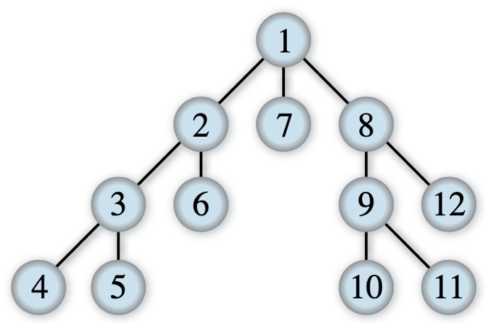
Fig. 58 Depth-first visit. Photo by Alexander Drichel, source: Wikipedia.

Accompany the implementation of the function with the appropriate test cases.

Solution to Exercise 61

from anytree import Node


# Test case for the function
def test_depth_first_visit(node, expected):
    result = depth_first_visit(node)
    if expected == result:
        return True
    else:
        return False


# Code of the function
def depth_first_visit(node):
    result = list()
    depth_first_visit_recursive(node, result)
    return result


def depth_first_visit_recursive(node, list):
    list.append(node)
    for child in node.children:
        depth_first_visit_recursive(child, list)


# Tests
n1 = Node(1)
n2 = Node(2, n1)
n3 = Node(3, n2)
n4 = Node(4, n3)
n5 = Node(5, n3)
n6 = Node(6, n2)
n7 = Node(7, n1)
n8 = Node(8, n1)
n9 = Node(9, n8)
n10 = Node(10, n9)
n11 = Node(11, n9)
n12 = Node(12, n8)
print(test_depth_first_visit(n1, [n1, n2, n3, n4, n5, n6, n7, n8, n9, n10, n11, n12]))

The source Python file of the code shown above is available as part of the material of the course. You can run it executing the command python ex-dev-depth_first_visit.py in a shell.

Exercise 62

Write in Python a function def breadth_first_visit(root_node) that does not use any recursion. This function takes a tree’s root node and returns a list of all nodes in breadth-first order. The breadth-first order considers all the nodes of the first level, then those ones of the second level, and so forth. For instance, considering the nodes created in the listing in Chapter “Organising information: trees”, the function called on the node book should return the following list:

[book, chapter_1, chapter_2, text_8, paragraph_1, paragraph_2, paragraph_3, text_7, text_1, quotation_1, text_3, quotation_2, text_5, text_6, text_2, text_4]

Accompany the implementation of the function with the appropriate test cases.

Solution to Exercise 62

from anytree import Node
from collections import deque


# Test case for the function
def test_breadth_first_visit(root_node, expected):
    result = breadth_first_visit(root_node)
    if expected == result:
        return True
    else:
        return False


# Code of the function
def breadth_first_visit(root_node):
    result = list()
    to_visit = deque()
    to_visit.append(root_node)

    while to_visit:
        node_to_visit = to_visit.popleft()
        result.append(node_to_visit)
        to_visit.extend(node_to_visit.children)

    return result


# Tests
book = Node("book")
chapter_1 = Node("chapter1", book)
chapter_2 = Node("chapter2", book)
paragraph_1 = Node("paragraph1", chapter_1)
text_1 = Node("text1", paragraph_1)
quotation_1 = Node("quotation1", paragraph_1)
text_2 = Node("text2", quotation_1)
text_3 = Node("text3", paragraph_1)
quotation_2 = Node("quotation2", paragraph_1)
text_4 = Node("text4", quotation_2)
paragraph_2 = Node("paragraph2", chapter_1)
text_5 = Node("text5", paragraph_2)
paragraph_3 = Node("paragraph3", chapter_1)
text_6 = Node("text6", paragraph_3)
text_7 = Node("text7", chapter_2)
text_8 = Node("text8", book)
bfv = [book,
       chapter_1, chapter_2, text_8,
       paragraph_1, paragraph_2, paragraph_3, text_7,
       text_1, quotation_1, text_3, quotation_2, text_5, text_6,
       text_2, text_4]
print(test_breadth_first_visit(book, bfv))

The source Python file of the code shown above is available as part of the material of the course. You can run it executing the command python ex-depth_first_visit.py in a shell.

Exercise 63

Write in Python a recursive version of the function defined in the {numref}´part-4-ex-13´.

Accompany the implementation of the function with the appropriate test cases.

Solution to Exercise 63

from anytree import Node
from collections import deque


# Test case for the function
def test_breadth_first_visit(root_node, expected):
    result = breadth_first_visit(root_node)
    if expected == result:
        return True
    else:
        return False


# Code of the function
def breadth_first_visit(root_node):
    result = list()

    if len(root_node.ancestors) == 0:  # It is the first call
        root_node.parent = Node(deque())

    queue = root_node.root.name
    result.append(root_node)
    queue.extend(root_node.children)

    if len(queue) > 0:
        result.extend(breadth_first_visit(queue.popleft()))
    else:
        root_node.root.children = ()

    return result


# Tests
book = Node("book")
chapter_1 = Node("chapter1", book)
chapter_2 = Node("chapter2", book)
paragraph_1 = Node("paragraph1", chapter_1)
text_1 = Node("text1", paragraph_1)
quotation_1 = Node("quotation1", paragraph_1)
text_2 = Node("text2", quotation_1)
text_3 = Node("text3", paragraph_1)
quotation_2 = Node("quotation2", paragraph_1)
text_4 = Node("text4", quotation_2)
paragraph_2 = Node("paragraph2", chapter_1)
text_5 = Node("text5", paragraph_2)
paragraph_3 = Node("paragraph3", chapter_1)
text_6 = Node("text6", paragraph_3)
text_7 = Node("text7", chapter_2)
text_8 = Node("text8", book)
bfv = [book,
       chapter_1, chapter_2, text_8,
       paragraph_1, paragraph_2, paragraph_3, text_7,
       text_1, quotation_1, text_3, quotation_2, text_5, text_6,
       text_2, text_4]
print(test_breadth_first_visit(book, bfv))

The source Python file of the code shown above is available as part of the material of the course. You can run it executing the command python ex-dev-depth_first_visit_recursive.py in a shell.

Exercise 64

A decision tree is a flowchart-like structure in which each internal node represents a test on an attribute (e.g. whether a coin flip comes up heads or tails), each branch represents the outcome of the test, and each leaf node represents a class label (i.e., a decision taken after computing all attributes). The paths from root to leaf represent classification rules. An example of a decision tree is shown in Fig. 59.

Fig. 59 Decision tree.

The decision tree above allows one to check whether a given number (identified by the variable attribute) is equal to 0. For checking this, supposing to execute such a decision tree passing the number 3 as input, one has (a) to start from the root, (b) to execute the condition (i.e. 3 < 0), (c) to follow the related branch (i.e. false), and (d) to repeat again the process if we arrived in an inner node or (e) to return the result if we arrived in a leaf node.

As shown in the figure, in a decision tree, each internal node always has two children: the left one is reached when the condition the internal node specifies is true, while the right one is reached when the condition the internal node specifies is false.

Write an algorithm in Python – def exec_dt(decision, attribute) – which takes in input a tree decision (which is represented by the root node of the tree defined as an object of the class anytree.Node) describing a decision tree, in which the name of each non-leaf node in the tree is a Python function – it means that we can see the node name as a function that can be executed by passing an input, e.g. considering the node n, we can call the function specified as its name passing the input between parenthesis, as usual: n.name(56). Each Python function, to execute using attribute as input, returns either True or False if the condition defined by that function is satisfied or is not satisfied, respectively. The algorithm returns the leaf node reached by executing the decision tree with the value in attribute.

Accompany the implementation of the function with the appropriate test cases.

Solution to Exercise 64

from anytree import Node


# Test case for the function
def test_exec_td(decision, attribute, expected):
    result = exec_td(decision, attribute)
    if expected == result:
        return True
    else:
        return False


# Code of the function
def exec_td(decision, attribute):
    if decision.children:
        if decision.name(attribute):
            return exec_td(decision.children[0], attribute)
        else:
            return exec_td(decision.children[1], attribute)
    else:
        return decision


# Tests
attr_equal = "attribute is equal to 0"
attr_not_equal = "attribute is not equal to 0"

root = Node(lambda x: x < 0)
root_left = Node(attr_not_equal, root)
root_right = Node(lambda x: x > 0, root)
root_right_left = Node(attr_not_equal, root_right)
root_right_right = Node(attr_equal, root_right)

print(test_exec_td(root, 0, root_right_right))
print(test_exec_td(root, 5, root_right_left))
print(test_exec_td(root, -10, root_left))

The source Python file of the code shown above is available as part of the material of the course. You can run it executing the command python ex-dev-decision_tree.py in a shell.

Exercise 65

A binary search tree is a binary tree data structure where each node may have at most two children, and the value of each node is greater than (or equal to) all the values in the respective node’s left subtree and less than (or equal to) the ones in its right subtree. It can be built, recursively following an approach which recalls the binary search strategy, starting from a list of ordered items (e.g. a list of integers), where each item becomes a node of a tree, as shown in Fig. 60.

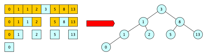
Fig. 60 Example of a binary search tree.

As a reminder, the binary search strategy first checks if the middle item of a list is equal to the item to search for and, in case this is not true, it continues to analyse the part of the list that either precedes or follows the middle item if it is greater than or less than the item to search.

Write a recursive algorithm in Python – def create_bst(ordered_list, parent) – which takes in input an ordered list of integers ordered_list and a parent node parent, and returns the root node of the binary search tree created from the input list. In the first call, the function is run passing None as input for the second parameter parent, e.g.

create_bst([0, 1, 1, 2, 3, 5, 8, 13], None)

and returns the binary search tree (i.e. its root node) shown in the example above.

Accompany the implementation of the function with the appropriate test cases.

Solution to Exercise 65

from anytree import Node, RenderTree

# Test case for the function
def test_create_bst(ordered_list, parent, expected):
    result = create_bst(ordered_list, parent)
    
    if str(RenderTree(result)) == str(RenderTree(expected)):
        return True
    else:
        return False


# Code of the function
def create_bst(ordered_list, parent):
    cur_len = len(ordered_list)

    if cur_len == 1:
        return Node(ordered_list[0], parent)
    elif cur_len > 1:
        mid = cur_len // 2
        
        r = Node(ordered_list[mid], parent)

        create_bst(ordered_list[:mid], r)
        create_bst(ordered_list[mid+1:], r)
        
        return r


# Tests
print(test_create_bst([9], None, Node(9)))

r1 = Node(5)
Node(1, r1)
Node(9, r1)
print(test_create_bst([1, 5, 9], None, r1))

r2 = Node(5)
r2_1 = Node(3, r2)
Node(1, r2_1)
r2_2 = Node(9, r2)
Node(7, r2_2)
print(test_create_bst([1, 3, 5, 7, 9], None, r2))

r3 = Node(3)
r3_1 = Node(1, r3)
r3_1_1 = Node(1, r3_1)
Node(0, r3_1_1)
Node(2, r3_1)
r3_2 = Node(8, r3)
Node(5, r3_2)
Node(13, r3_2)
print(test_create_bst([0, 1, 1, 2, 3, 5, 8, 13], None, r3))

The source Python file of the code shown above is available as part of the material of the course. You can run it executing the command python ex-dev-binary_search_tree.py in a shell.

Exercise 66

Propose some variation to the implementation of the peg solitaire exercise in Chapter “Backtracking algorithms” to make it more efficient – in particular, avoiding unsuccessful configurations if they have already been encountered previously while looking for a solution.

Accompany the implementation of the function with the appropriate test cases.

Solution to Exercise 66

from anytree import Node
from collections import deque


# Test case for the algorithm
def test_solve(pegs, holes, last_move, no_win_list, expected):
    result = solve(pegs, holes, last_move, no_win_list)
    if expected == result.name["in"] and len(pegs) == 1:
        return True
    else:
        return False


# Code of the algorithm
def solve(pegs, holes, last_move, no_win):
    result = None

    if pegs not in no_win:
        no_win.append(set(pegs))

        if len(pegs) == 1 and (5, 1) in pegs:  # leaf-win base case
            result = last_move
        else:
            last_move.children = valid_moves(pegs, holes)

            if len(last_move.children) == 0:  # leaf-lose base case
                undo_move(last_move, pegs, holes)  # backtracking
            else:  # recursive step
                possible_moves = deque(last_move.children)

                while result is None and len(possible_moves) > 0:
                    current_move = possible_moves.pop()
                    apply_move(current_move, pegs, holes)
                    result = solve(pegs, holes, current_move, no_win)

                if result is None:
                    undo_move(last_move, pegs, holes)  # backtracking
    else:
        undo_move(last_move, pegs, holes)  # backtracking

    return result


def create_board():
    initial_hole = (5, 1)
    holes = set()
    holes.add(initial_hole)

    pegs = set([
        (1, 0), (4, 0),
        (0, 1), (1, 1), (2, 1), (3, 1), (4, 1),
        (1, 2), (4, 2),
        (1, 3), (4, 3),
        (0, 4), (1, 4), (2, 4), (3, 4), (4, 4), (5, 4),
        (1, 5), (4, 5)
    ])

    return pegs, holes


def valid_moves(pegs, holes):
    result = list()

    for x, y in holes:
        if (x-1, y) in pegs and (x-2, y) in pegs:
            result.append(Node({"move": (x-2, y), "in": (x, y), "remove": (x-1, y)}))
        if (x+1, y) in pegs and (x+2, y) in pegs:
            result.append(Node({"move": (x+2, y), "in": (x, y), "remove": (x+1, y)}))
        if (x, y-1) in pegs and (x, y-2) in pegs:
            result.append(Node({"move": (x, y-2), "in": (x, y), "remove": (x, y-1)}))
        if (x, y+1) in pegs and (x, y+2) in pegs:
            result.append(Node({"move": (x, y+2), "in": (x, y), "remove": (x, y+1)}))

    return result


def apply_move(node, pegs, holes):
    move = node.name
    old_pos = move.get("move")
    new_pos = move.get("in")
    eat_pos = move.get("remove")

    pegs.remove(old_pos)
    holes.add(old_pos)

    pegs.add(new_pos)
    holes.remove(new_pos)

    pegs.remove(eat_pos)
    holes.add(eat_pos)


def undo_move(node, pegs, holes):
    move = node.name
    old_pos = move.get("move")
    new_pos = move.get("in")
    eat_pos = move.get("remove")

    pegs.add(old_pos)
    holes.remove(old_pos)

    pegs.remove(new_pos)
    holes.add(new_pos)

    pegs.add(eat_pos)
    holes.remove(eat_pos)


# Tests
pegs, holes = create_board()
print(test_solve(pegs, holes, Node("start"), list(), (5, 1)))

The source Python file of the code shown above is available as part of the material of the course. You can run it executing the command python ex-solve_dp.py in a shell.

Exercise 67

AtariGo is a simplified version of Go. Its rules are pretty simple. Two teams, Black and White, take turns placing a stone (game piece) of their own colour on a vacant point (intersection) of the grid on the board. Once placed, stones do not move. A vacant point adjacent to a stone is called a liberty for that stone. Connected stones formed a group and shared their liberties. A stone or group with no liberties is captured. Black plays first. The first team to capture anything wins.

Suppose you want to develop software that can play AtariGo on a 4x4 board, as shown in Fig. 61, already populated with some stones.

Fig. 61 An example of a small Go board.

Suppose we use tuples to define every position in the board, as shown as follows:

(0, 0) (1, 0) (2, 0) (3, 0)
(0, 1) (1, 1) (2, 1) (3, 1)
(0, 2) (1, 2) (2, 2) (3, 2)
(0, 3) (1, 3) (2, 3) (3, 3)

One of the functions to implement returns the set of board positions that are not occupied by any stone and that do not result in the stone being immediately captured if placed. Supposing White has to play on the board in the figure, such a function would return the set containing the tuples (0, 0), (1, 0) and (0, 1) – but not (3, 3) since if White places a stone there it will be immediately captured.

Write a function in Python – def get_good_white_moves(white, black) – that takes in input the set of tuples identifying the stones placed in the 4x4 board in the previous turns by the two players (white and black, respectively) and that returns the set of all the tuples identifying possible places where White can put its stone in the current turn, according to the rules mentioned above. As a simplification, avoid checking the liberties of groups of White stones.

Accompany the implementation of the function with the appropriate test cases.

Solution to Exercise 67

# Test case for the function
def test_get_good_white_moves(white, black, expected):
    result = get_good_white_moves(white, black)
    if expected == result:
        return True
    else:
        return False


# Code of the function
def get_good_white_moves(white, black):
    result = set([
        (0, 0), (1, 0), (2, 0), (3, 0),
        (0, 1), (1, 1), (2, 1), (3, 1),
        (0, 2), (1, 2), (2, 2), (3, 2),
        (0, 3), (1, 3), (2, 3), (3, 3)
    ])
    result.difference_update(white)
    result.difference_update(black)

    for x, y in set(result):
        if not have_freedom((x - 1, y), black) and not have_freedom((x + 1, y), black) and \
                not have_freedom((x, y - 1), black) and not have_freedom((x, y + 1), black):
            result.remove((x, y))

    return result


def have_freedom(t, black):
    return 0 <= t[0] <= 3 and 0 <= t[1] <= 3 and t not in black


# Tests
print(test_get_good_white_moves(
    {(1, 1), (0, 2), (0, 3), (1, 0)},
    {(2, 0), (2, 1), (3, 1), (2, 2), (2, 3)},
    {(0, 0), (0, 1), (1, 2), (1, 3), (3, 2), (3, 3)}))

The source Python file of the code shown above is available as part of the material of the course. You can run it executing the command python ex-dev-atari_go.py in a shell.

Exercise 68

We define a labyrinth as a set of tuples representing the cells of its paths. The tuples are organised in an x/y grid, similar to the way used in the listing in Chapter “Backtracking algorithms” for the peg solitaire, such as the one proposed as follows:

      (1,0)       (3,0) (4,0) (5,0)
(0,1) (1,1) (2,1) (3,1)       (5,1)
(0,2)       (2,2)       (4,2) (5,2)
(0,3)       (2,3) (3,3)       (5,3)
(0,4)                   (4,4)      
(0,5) (1,5) (2,5) (3,5) (4,5)      

Write the function solve_labyrinth(paths, entrance, exit, last_move) using a backtracking approach, which takes as input the paths of the labyrinth (such as the ones mentioned above), two tuples representing the entrance and the exit of the labyrinth, and the last move made. The function returns the last move done to reach the exit if the labyrinth has an escape; otherwise, it returns None.

Accompany the implementation of the function with the appropriate test cases.

Solution to Exercise 68

from anytree import Node
from collections import deque


# Test case for the function
def test_solve_labyrinth(paths, entrance, exit, last_move, expected):
    result = solve_labyrinth(paths, entrance, exit, last_move)
    if result is not None and result.name == exit:
        return True
    else:
        return False


# Code of the function
def solve_labyrinth(paths, entrance, exit, last_move):
    result = None
    paths.remove(last_move.name)

    if entrance == exit:  # leaf-win base case
        result = last_move
    else:
        last_move.children = valid_moves(paths, entrance[0], entrance[1])

        if len(last_move.children) == 0:  # leaf-lose base case
            paths.add(last_move.name)  # backtracking
        else:  # recursive step
            possible_moves = deque(last_move.children)

            while result is None and len(possible_moves) > 0:
                current_move = possible_moves.pop()
                result = solve_labyrinth(paths, current_move.name, exit, current_move)

            if result is None:
                paths.add(last_move.name)  # backtracking

    return result


def create_labyrinth():
    return set([
        (1, 0), (3, 0), (4, 0), (5, 0),
        (0, 1), (1, 1), (2, 1), (3, 1), (5, 1),
        (0, 2), (2, 2), (4, 2), (5, 2),
        (0, 3), (2, 3), (3, 3), (5, 3),
        (0, 4), (4, 4),
        (0, 5), (1, 5), (2, 5), (3, 5), (4, 5)])


def valid_moves(available_paths, x, y):
    result = list()

    if (x - 1, y) in available_paths:
        result.append(Node((x - 1, y)))
    if (x + 1, y) in available_paths:
        result.append(Node((x + 1, y)))
    if (x, y - 1) in available_paths:
        result.append(Node((x, y - 1)))
    if (x, y + 1) in available_paths:
        result.append(Node((x, y + 1)))

    return result


# Tests
print(test_solve_labyrinth(create_labyrinth(), (1, 0), (5, 3), Node((1, 0)), (5, 3)))
print(test_solve_labyrinth(create_labyrinth(), (5, 3), (1, 0), Node((5, 3)), (1, 0)))
print(test_solve_labyrinth(create_labyrinth(), (1, 0), (1, 0), Node((1, 0)), (1, 0)))

The source Python file of the code shown above is available as part of the material of the course. You can run it executing the command python ex-solve_labirinth.py in a shell.

Exercise 69

A minimax is a recursive algorithm for choosing the next move in a two-player (A and B) game like chess, where all the possible configurations of the board are described as nodes in a tree of moves. A value is associated with each configuration (i.e. each node) and indicates how good it would be for a player (either A or B, depending on the turn) to reach that configuration. If it is A’s turn to move, A gives a value to each of its legal moves, i.e. the child nodes of the one describing the current configuration. The best value for A is the maximum of the values of the children of the configuration in which A has to play, while the best value for B is the minimum of the values of the children of the configuration in which B has to play.

The minimax uses a heuristic function get_value only when a terminal node of the tree of moves is reached or when nodes at the maximum search depth are reached (the maximum depth is specified as input to the algorithm). The other non-leaf nodes inherit their value from a descendant leaf/max-depth node, i.e. either the maximum of the values of the children if A is playing or the minimum of the values of the children if B is playing. An example of minimax execution is shown in Fig. 62.

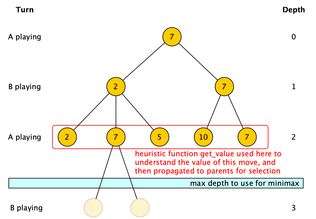
Fig. 62 Minimax execution.

Write an algorithm in Python – def minimax(node, max_depth, player_a_moves) – which takes in input a node of the tree of moves, the maximum depth to consider while visiting the tree of moves, and whether the player A is playing (when player_a_moves is True) or its opponent is (when player_a_moves is False), and returns the heuristic value that will be assigned to the input node. The function def get_value(node), for getting the heuristic value associated with a leaf or a node at maximum depth, and another function def get_next_valid_moves(node), used to get all the moves (i.e. children) of a configuration (i.e. a node), are provided (i.e. they must not be developed) and can be directly used in the implementation of the algorithm. Initially, for instance considering the image above, the algorithm will be called as follows:

minimax(root, 2, True)

Accompany the implementation of the function with the appropriate test cases.

Solution to Exercise 69

from anytree import Node


# Test case for the function
def test_minimax(node, max_depth, player_a_moves, expected):
    result = minimax(node, max_depth, player_a_moves)
    if expected == result:
        return True
    else:
        return False


# Code of the function
def minimax(node, max_depth, player_a_moves):
    if max_depth == 0 or len(node.children) == 0:
        return get_value(node)
    else:
        move_values = []
        for move in get_next_valid_moves(node):
            move_values.append(minimax(move, max_depth - 1, not player_a_moves))
            
        if player_a_moves:
            return max(move_values)
        else:
            return min(move_values)


# Ancillary functions for granted
def get_value(node):
    d = {
        "Move X": 2,
        "Move Y": 7,
        "Move Z": 5,
        "Move W": 10,
        "Move V": 8
    }
    return d[node.name]


def get_next_valid_moves(node):
    return node.children


# Tests
root = Node("Move Y")
node_1_1 = Node("Move X", root)
node_1_2 = Node("Move Y", root)
node_2_1 = Node("Move X", node_1_1)
node_2_2 = Node("Move Y", node_1_1)
node_2_3 = Node("Move Z", node_1_1)
node_2_4 = Node("Move W", node_1_2)
node_2_5 = Node("Move Y", node_1_2)
node_3_1 = Node("Move Y", node_2_2)
node_3_2 = Node("Move V", node_2_2)

print(test_minimax(root, 0, True, 7))
print(test_minimax(root, 2, True, 7))
print(test_minimax(root, 3, True, 7))
print(test_minimax(root, 7, True, 7))

The source Python file of the code shown above is available as part of the material of the course. You can run it executing the command python ex-dev-minimax.py in a shell.

Exercise 70

Consider the list of co-authors of Tim Berners-Lee as illustrated in the right box at http://dblp.uni-trier.de/pers/hd/b/Berners=Lee:Tim. Build an undirected graph that contains Tim Berners Lee as the central node, and that links to five nodes representing his top-five co-authors. Also, specify the weight of each edge as an attribute, where the value of the weight is the number of bibliographic resources (articles, proceedings, etc.) Tim Berners-Lee has co-authored with the person linked by that edge.

Solution to Exercise 70

from networkx import Graph

g = Graph()

g.add_node("Tim Berners-Lee")
g.add_node("Tom Heath")
g.add_node("Christian Bizer")
g.add_node("Sören Auer")
g.add_node("Lalana Kagal")
g.add_node("Daniel J. Weitzner")

g.add_edge("Tim Berners-Lee", "Tom Heath", weight=18)
g.add_edge("Tim Berners-Lee", "Christian Bizer", weight=18)
g.add_edge("Tim Berners-Lee", "Sören Auer", weight=10)
g.add_edge("Tim Berners-Lee", "Lalana Kagal", weight=9)
g.add_edge("Tim Berners-Lee", "Daniel J. Weitzner", weight=8)

The source Python file of the code shown above is available as part of the material of the course. You can run it executing the command python ex-graph.py in a shell.

Exercise 71

Create a directed graph which relates the actors Brad Pitt, Eva Green, George Clooney, Catherine Zeta-Jones, Johnny Depp, and Helena Bonham Carter to the following movies: Ocean’s Twelve, Fight Club, Dark Shadows.

Solution to Exercise 71

from networkx import DiGraph

g = DiGraph()

g.add_node("Brad Pitt")
g.add_node("Eva Green")
g.add_node("George Clooney")
g.add_node("Catherine Zeta-Jones")
g.add_node("Johnny Depp")
g.add_node("Helena Bonham Carter")
g.add_node("Ocean's Twelve")
g.add_node("Fight Club")
g.add_node("Dark Shadows")

g.add_edge("Brad Pitt", "Ocean's Twelve")
g.add_edge("George Clooney", "Ocean's Twelve")
g.add_edge("Catherine Zeta-Jones", "Ocean's Twelve")

g.add_edge("Brad Pitt", "Fight Club")
g.add_edge("Helena Bonham Carter", "Fight Club")

g.add_edge("Helena Bonham Carter", "Dark Shadows")
g.add_edge("Johnny Depp", "Dark Shadows")
g.add_edge("Eva Green", "Dark Shadows")

The source Python file of the code shown above is available as part of the material of the course. You can run it executing the command python ex-digraph.py in a shell.

Exercise 72

The Erdős number quantifies the collaborative distance between the mathematician Paul Erdős and another person, measured by the number of scholarly articles they have co-authored. In practice, having the collaboration network of some people described as an undirected graph, where each node represents a person and an edge between two people states that they have coauthored some article together, the goal is to find the minimal distance, computed as the number of edges to traverse, between the node representing Paul Erdős and another input person.

An Erdős number by research group (ENG) is the average number computed by dividing the Erdős numbers of each member of the research group by the number of people in that group.

Write an algorithm in Python – def eng(coauthor_graph, research_group) – which takes in input an undirected graph coauthor_graph (i.e. an object of the class networkx.Graph) describing a collaboration network, in which each node is defined by the string of the name of a person and that includes the node "Paul Erdős", and the list of strings research_group, which contains the strings of the names of people that are member of a research group. The Python function should return the Erdős number for the corresponding research group.

Accompany the implementation of the function with the appropriate test cases.

Solution to Exercise 72

from networkx import Graph


# Test case for the function
def test_eng(coauthor_graph, research_group, expected):
    result = eng(coauthor_graph, research_group)
    if expected == result:
        return True
    else:
        return False


# Code of the function
def eng(coauthor_graph, research_group):
    erdos = dict()
    for node in coauthor_graph.nodes:
        erdos[node] = 0

    to_visit = ["Paul Erdős"]
    to_visit.extend(coauthor_graph.adj["Paul Erdős"])
    idx = 1

    while idx < len(to_visit):
        node = to_visit[idx]
        idx = idx + 1
        erdos[node] = erdos[node] + 1
        
        for child in coauthor_graph.adj[node]:
            if child not in to_visit:
                erdos[child] = erdos[child] + erdos[node]
                to_visit.append(child)
    
    total = 0
    for member in research_group:
        total = total + erdos[member]
    
    return total / len(research_group)


# Tests
g = Graph()
pe = "Paul Erdős"
ad = "Alice Doe"
bd = "Bob Doe"
cd = "Charles Doe"
dd = "Des Doe"
ed = "Estella Doe"

g.add_edge(pe, ad)
g.add_edge(ad, bd)
g.add_edge(ad, cd)
g.add_edge(bd, cd)
g.add_edge(bd, dd)
g.add_edge(bd, ed)
g.add_edge(ad, ed)

print(test_eng(g, [pe], 0))
print(test_eng(g, [ad], 1))
print(test_eng(g, [bd], 2))
print(test_eng(g, [ed], 2))
print(test_eng(g, [dd], 3))
print(test_eng(g, [ad, bd, ed, dd], 2))

The source Python file of the code shown above is available as part of the material of the course. You can run it executing the command python ex-dev-erdos.py in a shell.

Exercise 73

A* is a search algorithm for weighted graphs. Starting from a specific start node of a graph, it aims to find a path to the given goal node having the smallest cost (i.e. the least distance travelled, considering the sum of the weights of all the edges crossed from start to goal). Typical implementations of A* use a priority queue to perform the repeated selection of minimum cost nodes to expand, computed using the following formula:

f(n) = g(n) + h(n)

where n is the next node on the path, g(n) is the cost of the path from the start node to n, and h(n) is a heuristic function (h is provided as input of the algorithm) that estimates the cost of the cheapest path from n to the goal.

At the very beginning of the algorithm, the priority queue is initialised with the start node, and f(start) is set to h(start). At each step of the algorithm, the node n with the lowest f(n) value is removed from the priority queue, the f and g values of its neighbours are updated accordingly, and these neighbours are added to the priority queue. The algorithm continues until the node with the lowest f value in the queue is removed (i.e., the goal node), at which point g(goal) is returned.

Write an algorithm in Python – def a_star(graph, start, goal, h) – which takes in input a directed graph (defined according to the networkx library), a start node in the graph, a goal node in the graph, and the function h used to compute f, and returns the cost of the cheapest path from start to goal. All the edges in the graph have specified an attribute weight (an integer) representing the cost to traverse that edge.

Accompany the implementation of the function with the appropriate test cases.

Solution to Exercise 73

from collections import deque
from networkx import Graph

# Test case for the function
def test_a_star(graph, start, goal, h, expected):
    result = a_star(graph, start, goal, h)
    if expected == result:
        return True
    else:
        return False


# Code of the function
def a_star(graph, start, goal, h):
    q = []
    q.append(start)
    f = {start: h(start)}
    g = {start: 0}

    while q:
        idx = select_item(q, f)
        item = q[idx]
        q.remove(item)

        if item == goal:
            return g[item]
        else:
            for node in graph.adj[item]:
                weight = graph.get_edge_data(item, node)["weight"]
                tmp_g = g[item] + weight
                if node not in g or tmp_g < g[node]:
                    g[node] = tmp_g
                    f[node] = g[node] + h(node)
                    q.append(node)
            
    return None

def select_item(q, f):
    f_values = []
    min_value = None

    for item in q:
        cur_value = f[item]
        f_values.append(cur_value)
        if min_value is None or cur_value < min_value:
            min_value = cur_value
        
    return f_values.index(min_value)

# Tests
g = Graph()
g.add_edge("a", "b", weight=2)
g.add_edge("b", "c", weight=3)
g.add_edge("c", "end", weight=4)
g.add_edge("end", "e", weight=2)
g.add_edge("e", "d", weight=3)
g.add_edge("d", "start", weight=2)
g.add_edge("start", "a", weight=1.5)

def my_h(x):
    res = {
        "start": 7,
        "a": 4,
        "b": 2,
        "c": 4,
        "d": 4.5,
        "e": 2,
        "end": 0
    }

    return res[x]

print(test_a_star(g, "start", "end", my_h, 7))
print(test_a_star(g, "start", "end", lambda x: 0, 7))

The source Python file of the code shown above is available as part of the material of the course. You can run it executing the command python ex-dev-a_star.py in a shell.

Exercise 74

PageRank is an algorithm used by Google Search to rank web pages in their search engine results. It operates on a directed graph where nodes represent webpages, and each directed edge represents a link from a source webpage to a target webpage. Each node of the graph has an associated PageRank that measures its relative importance within the graph (the greater, the more critical).

In its simplified version, it is computed as follows. It takes as input a directed graph, where each node has a potential PageRank transfer value to share with other nodes, initialised to 1. Then, the algorithm transfers the potential value of a given node to its outbound targets, dividing it equally among all outbound links. For instance, suppose that page B had a link to pages C and A, page C has a link to page A, and page D has links to all three pages. Thus, page B would transfer half of its existing value (0.5) to page A and the other half (0.5) to page C. Page C would transfer all of its existing value (1) to the only page it links to, A. Since D had three outbound links, it would transfer one third of its existing value, or approximately 0.33, to A, B and C. The sum of all the values that are transferred to a given node is the PageRank of that node – for instance, page A will have a PageRank of approximately 1.83.

Write an algorithm in Python – def simplified_pr(g) – which takes in input a directed graph created using the networkx library, and returns a dictionary having as many key-value pairs as the number of nodes in the graph. In particular, each pair maps a node name to its PageRank. It is possible to use the method adj[n] of a graph for getting all the nodes reachable from a node n by following its outbound edges. For instance, in the example above, where the graph is stored as a DiGraph in the variable my_g, my_g.adj["D"] returns a collection containing the nodes A, B, and C.

Accompany the implementation of the function with the appropriate test cases.

Solution to Exercise 74

from networkx import DiGraph


# Test case for the function
def test_simplified_pr(g, expected):
    result = simplified_pr(g)
    
    if len(result) == len(expected):
        test_res = True
        for key in result:
            if round(result[key], 2) != round(expected[key], 2):
                test_res = False
        return test_res
    else:
        return False


# Code of the function
def simplified_pr(g):
    result = {}

    for n in g.nodes:
        if n not in result:
            result[n] = 0
        
        adj_n = g.adj[n]

        if len(adj_n):
            value = 1 / len(adj_n)

            for a in adj_n:
                if a not in result:
                    result[a] = 0
                result[a] += value

    return result
    
            
# Tests
my_g = DiGraph()
my_g.add_edge("B", "C")
my_g.add_edge("B", "A")
my_g.add_edge("C", "A")
my_g.add_edge("D", "A")
my_g.add_edge("D", "B")
my_g.add_edge("D", "C")

res = {
    "A": 1.83,
    "B": 0.33,
    "C": 0.83,
    "D": 0
}

print(test_simplified_pr(my_g, res))

The source Python file of the code shown above is available as part of the material of the course. You can run it executing the command python ex-dev-pagerank.py in a shell.

Exercise 75

Implement the algorithm introduced in Section “The greedy algorithmic approach” of Chapter “Greedy algorithms” for returning the minimum amount of coins for a change.

Accompany the implementation of the function with the appropriate test cases.

Solution to Exercise 75

# Test case for the function
def test_return_change(amount, expected):
    result = return_change(amount)
    if expected == result:
        return True
    else:
        return False


# Code of the function
def return_change(amount):
    result = dict()
    coins = [2.0, 1.0, 0.5, 0.2, 0.1, 0.05, 0.02, 0.01]

    for coin in coins:
        while float_diff(amount, coin) >= 0:
            amount = float_diff(amount, coin)

            if coin not in result:
                result[coin] = 0
            result[coin] = result[coin] + 1

    return result


# The use of the 'round' function is justified due to the precision in the representation
# of floating point numbers, see https://docs.python.org/3/tutorial/floatingpoint.html.
def float_diff(f1, f2):
    return round(f1 - f2, 2)


# Tests
print(test_return_change(5.00, {2.0: 2, 1.0: 1}))
print(test_return_change(2.76, {2.0: 1, 0.5: 1, 0.2: 1, 0.05: 1, 0.01: 1}))
print(test_return_change(0.00, {}))

The source Python file of the code shown above is available as part of the material of the course. You can run it executing the command python ex-return_change.py in a shell.

Exercise 76

Suppose one must schedule the maximum number of activities in a day, choosing from a set of available activities, while one can address at most one activity at a time. Each activity is defined by a tuple, where the first element specifies the start time (an integer from 0 to 24, indicating the start hour), and the second element specifies the finish time (an integer from 0 to 24, indicating the finish hour). Develop the Python function def select_activities(set_of_activities) by using a greedy approach. It takes as input a set of day-level activities and returns the list of the maximum number of non-overlapping activities that can be scheduled, ordered by start time. Hint: consider each activity’s finish time and how it may affect the selection.

Accompany the implementation of the function with the appropriate test cases.

Solution to Exercise 76

from collections import deque


# Test case for the function
def test_select_activities(set_of_activities, expected):
    result = select_activities(set_of_activities)
    if expected == len(result):
        bool_result = True
        for idx, activity in enumerate(result):
            if idx > 0:
                bool_result = bool_result and (activity[0] >= result[idx - 1][1])

        return bool_result
    else:
        return False


# Code of the function
def select_activities(set_of_activities):
    ordered_activities = deque()
    for activity in set_of_activities:
        insert_position = len(ordered_activities)
        for idx in reversed(range(insert_position)):
            if activity[1] < ordered_activities[idx][1]:
                insert_position = idx
        ordered_activities.insert(insert_position, activity)

    result = list()
    finish_time = 0
    while len(ordered_activities) > 0:
        activity = ordered_activities.popleft()
        if activity[0] >= finish_time:
            result.append(activity)
            finish_time = activity[1]

    return result


# Tests
activities_1 = set()
activities_1.add((0, 3))
activities_1.add((4, 7))
activities_1.add((2, 12))
activities_1.add((7, 8))
activities_1.add((10, 13))
activities_1.add((12, 20))
activities_1.add((14, 17))
activities_1.add((16, 19))
activities_1.add((17, 24))
activities_1.add((21, 23))
print(test_select_activities(activities_1, 6))
print(test_select_activities(set(), 0))

The source Python file of the code shown above is available as part of the material of the course. You can run it executing the command python ex-select_activities.py in a shell.

Exercise 77

Graph colouring is an assignment of attributes traditionally called “colours” to the vertices of an undirected graph subject to certain constraints, where no two adjacent vertices are of the same colour, as shown in Fig. 63.

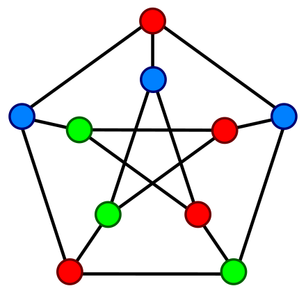
Fig. 63 Example of a graph colouring.

A greedy colouring is a colouring of the vertices of a graph formed by a greedy algorithm that considers the vertices of the graph in sequence and assigns each vertex its first available colour. The algorithm processes the vertices, assigning a colour to each one as it is processed. The colours should be represented by the non-negative integers 0, 1, 2, etc., and each vertex is given the colour with the smallest colour number that is not already used by one of its neighbours.

Write an algorithm in Python – def greedy_colouring(g) – that implements the greedy colouring, which takes in input an undirected graph g, created using the library networkx, and returns a dictionary having the name of the vertex as key and the non-negative integer defining its colour as value. Important: having a graph g, the method g.neighbors(n) returns an iterator (acting as a list, when used in a for each loop) of all the neighbours of the given node n.

Accompany the implementation of the function with the appropriate test cases.

Solution to Exercise 77

from networkx import Graph

# Test case for the function
def test_greedy_colouring(g, expected):
    result = greedy_colouring(g)
    
    if result == expected:
        return True
    else:
        return False


# Code of the function
def greedy_colouring(g):
    result = dict()

    for node in g.nodes:
        colour = 0
        used = set()

        for nei in g.neighbors(node):
            if nei in result:
                used.add(result[nei])
        
        while colour in used:
            colour += 1
        
        result[node] = colour
    
    return result


# Tests   
my_g = Graph()
my_g.add_edge(1, 2)
my_g.add_edge(2, 3)
my_g.add_edge(3, 4)
my_g.add_edge(4, 5)
my_g.add_edge(5, 1)
my_g.add_edge(1, 6)
my_g.add_edge(2, 7)
my_g.add_edge(3, 8)
my_g.add_edge(4, 9)
my_g.add_edge(5, 10)
my_g.add_edge(6, 8)
my_g.add_edge(6, 9)
my_g.add_edge(7, 9)
my_g.add_edge(7, 10)
my_g.add_edge(8, 10)

result = {
    1: 0,
    2: 1,
    3: 0,
    4: 1,
    5: 2,
    6: 1,
    7: 0,
    8: 2,
    9: 2,
    10: 1 
}

print(test_greedy_colouring(my_g, result))

The source Python file of the code shown above is available as part of the material of the course. You can run it executing the command python ex-dev-colouring.py in a shell.

References

[Fblinry18a]

Sándor P. Fekete and blinry. BINÄRY SEARCH. February 2018. URL: https://idea-instructions.com/binary-search/.

[Fblinry18b]

Sándor P. Fekete and blinry. KVICK SÖRT. March 2018. URL: https://idea-instructions.com/quick-sort/.